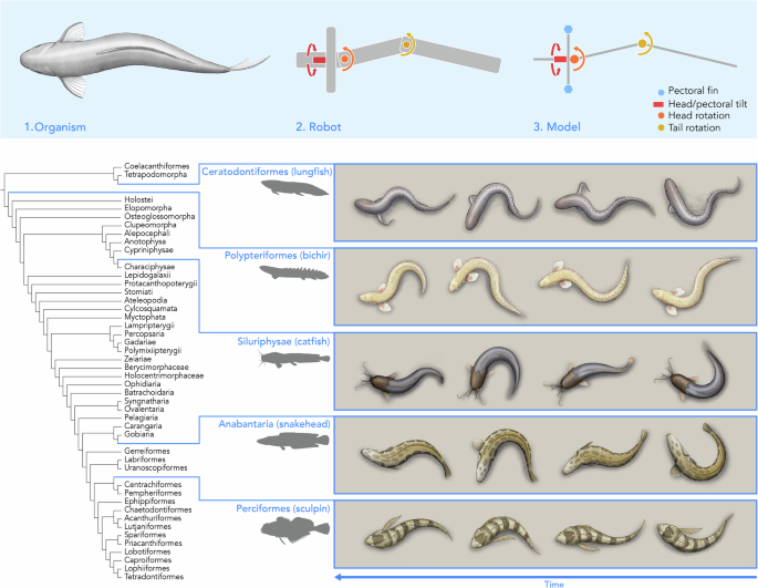
The undulating tripod gait as a model of the locomotion of walking fish

Definition of the undulating tripod gait model

The undulating tripod gait can be described as a coordinated combination of two motions: a propping action generated by an anterior body part, such as a pectoral fin, and a pushing action produced by the posterior body, including the axial musculature and caudal region. During locomotion, the fish alternates which side of the body makes contact with the substrate, using ground reaction forces to rotate its body around the planted prop. When the body is propped on the left side of the midline, the fish swings around the pivot point in the counterclockwise direction and vice versa when the body is propped on the right side of the midline (Fig. 2). The time series of postures within a gait cycle depends on the exact morphology and gait parameters; rather, it is the sequence of these general actions that defines the undulating tripod gait (Fig. 1).

Fig. 2: The simplified model of the undulating tripod gait, where the soft body of the fish is discretized into three rigid segments that rotate with respect to each other. The alternative text for this image may have been generated using AI. Full size image The blue hexagons indicate the pectoral fins, where the dark blue specifically indicates contact with the ground. The red box indicates the head and pectoral tilt θ 1 (rotation in roll, aligned in the anterior-posterior direction), the orange circle indicates the head rotation θ 2 (rotation in yaw, aligned in the dorsal-ventral direction), and the yellow circle indicates the tail rotation θ 3 (rotation in yaw, aligned in the dorsal-ventral direction). The schematics are not linked to specific timesteps, as the postures of the fish within its gait cycle depend on the exact gait parameters.

To explore the principles of the undulating tripod gait, we created a simple theoretical model that recreates these salient features. In this model (Fig. 2), we represent the propping motion as being generated by a rigid beam rotating around the fish’s head-tail axis (θ 1 ) such that θ 1 > 0 pushes the beam into the surface on the left side of the body. We approximate the continuum soft body as three rigid beams (lengths L 1 , L 2 , and L 3 from head to tail, respectively) connected by two revolute joints (θ 2 between the head and center links and θ 3 between the center and tail links) whose axes are both normal to the plane of the substrate on which the fish is walking. The rotations of θ 2 and θ 3 create the pushing motion that swings the body around the pivot point engaged with the surface. We refer to this as an undulating tripod gait because, under the model’s kinematic constraints, the fish maintains contact with the ground at three key points: the tip of the propping beam and two locations along the body segments.

The precise positions of these contact points are not fixed but instead emerge from the fish’s body shape and mass distribution. In this model, locomotion results only from the interplay of gravitational forces, joint trajectories, and friction-dominated contact with the substrate.

Analysis of biological inspirations

In this work, we focus specifically on the terrestrial locomotion of Polypterus senegalus as an exemplar of the undulating tripod gait, in which the fish uses its pectoral fins as propping appendages (Supplementary Movie 1). P. senegalus is a species of fish capable of surviving in both aquatic and terrestrial environments, and its ability to live on land for extended periods of time has led to a significant literature on its terrestrial walking gaits27,33,34. Furthermore, its long, slender, flexible body is capable of significant axial bending, which potentially provides a larger feasible space of possible gait patterns compared to fish with stiffer axial columns.

We tracked the motion of six specimens across at least one complete gait cycle, defined as beginning and ending with the tail at its maximal rightward bend, to extract key parameters of the gait and body morphology for use in simulations and physical modeling. To approximate P. senegalus within the framework of the undulating tripod gait model introduced above, we digitized the midline of the body over time (Fig. 3a) and fit it using three connected linear segments (see “Methods” for more details). Based on observations of the walking motion, the lengths of these segments followed a 2:4:5 ratio, corresponding to 0.182, 0.367, and 0.455 of the body length (BL). With this ratio, the first joint was positioned near the pectoral girdle, as we observed little bending to the anterior of that point, and the second joint was placed slightly ahead of the pelvic girdle to capture both bending in the body and in the tail. Using this discretization, we observed that the angular motions at joints θ 2 and θ 3 exhibited approximately sinusoidal trajectories during periods of steady locomotion. Although gait frequency varied across individuals, each trial contained intervals of consistent timing and waveform shape sufficient for reliable sinusoidal fitting (Fig. 3e, f). The resulting amplitude and phase parameters are reported in Table 1 and served as input for both the simulated and physical robot models.

Fig. 3: Tracking of the walking motion of Polypterus senegalus. The alternative text for this image may have been generated using AI. Full size image a Time series images of one cycle of P. senegalus’s gait with the tracked midline overlaid (red). b Time series images of one gait cycle with the discretization of the body into three linear segments overlaid. The three-segment discretization is denoted by blue (head segment), green (body segment), and pink (tail segment) lines. Scale bar is 5 cm. c Comparison of the theoretical tripod gait model to d the three-segment discretization. e Fitting a sinusoid to θ 2 , the joint between the head and body segments, and f fitting a sinusoid to θ 3 , the joint between the body and tail segments, where each trial is plotted in gray, the average of the four trials is plotted in solid color, and the fitted sinusoid is plotted as a dashed line.

Table 1 Fitted sinusoidal parameters identified from the observations of P. senegalus Full size table

We found that this general gait pattern describes the walking locomotion of a diversity of fish species with different morphologies including those we highlighted in Fig. 1. We tracked the midlines (see “Methods” for more details) of five different fish that exhibit the undulating tripod gait: P. senegalus, the African lungfish Protopterus annectens35, several species of catfish Pterygoplichthys disjunctivus, Pterygoplichthys multiradiatus, Pterygoplichthys gibbiceps, Hoplosternum punctatus, and Hoplosternum sp.36,37, the northern snakehead Channa argus38, and the tidepool sculpin Oligocottus maculosus39 (Fig. 4a). We split the continuous walking behavior into individual gait cycles starting and ending with the tail to the right side of the fish’s body and averaged the per-cycle observations. We took the anterior point of the head as the primary propping point for P. annectens and the pectoral fins as the primary propping points for the other species. Across species, all the fish alternate which side of the body makes contact with the substrate and subsequently sweep the tail toward that planted side (i.e., after engaging the left pectoral fin, the tail bends leftward). Although the timing of individual movements and the location of the propping structure vary among species and specimens, the overall sequence of prop, bend, and pivot remains consistent within the undulating tripod gait. The gait pattern is generally symmetric (Fig. 4e).

Fig. 4: Comparison of the walking kinematics of five fish species exhibiting the undulating tripod gait. The alternative text for this image may have been generated using AI. Full size image a Illustrations of the five species - the African lungfish Protopterus annectens, the gray bichir P. senegalus, several species of catfish Pterygoplichthys disjunctivus, Pterygoplichthys multiradiatus, Pterygoplichthys gibbiceps, Hoplosternum punctatus, and Hoplosternum sp., the northern snakehead Channa argus, and the tidepool sculpin Oligocottus maculosus. b Angular position of the first body joint over the course of one gait cycle for each of the fish species. c Angular position of the second body joint over the course of one gait cycle for each of the fish species. The lighter traces denote each gait cycle tracked, and the dark, bolded traces are the average of the tracked gait cycles. The number of specimens for each are n = 2 (lungfish), n = 6 (bichir), n = 5 (catfish), n = 4 (snakehead), n = 1 (sculpin). d Diagram of the discretization overlaid on an illustration of the bichir, where the dotted line denotes an extension of the middle segment to define the angles θ 2 and θ 3 . e Gait diagram of the walking locomotion of the five species, divided into the movement of the tail and the propping anterior contact between the fish and the surface. More details can be found in the Supplementary Information.

Similarly, when these species were approximated using the same discretization into three rigid segments (see “Methods” for more details), the trajectories of θ 2 (Fig. 4b) and θ 3 (Fig. 4c) exhibited consistent sinusoidal patterns. While the amplitude of joint motion varied among species, the phase relationship between the time series trajectories of θ 2 and θ 3 remained conserved. This is strong evidence that the walking gaits of these species can all be described by the undulating tripod gait model, with P. senegalus serving as an exemplar.

Simulating morphology and motion

To systematically evaluate the locomotion of a system under the constraints imposed by our model, we created a simulation of a robot that uses the undulating tripod gait. The simulation is inspired by the morphology and gait kinematics of P. senegalus and subject to the approximations made in our model of the undulating tripod gait. We used this simulation to investigate parameters of both the morphology and the gait that were not observed in our experiments with real fish and to determine how these parameters affect walking locomotion (see “Methods” for more details).

In our simulation, the fish’s body was represented by three rigid links that rotate with respect to each other in the same plane via revolute joints. From the tracking of the fish described in Fig. 3, the head, middle, and tail segments have lengths of a 2:4:5 ratio, with an overall length of 0.1 m, similar to the length scale of P. senegalus. These joints were controlled by time-series angular position inputs, and the robot is driven forward by the interactions between the robot and the ground, calculated by the simulation environment. Here, we assume that there is sufficient capacity for torque generation in each of the joints to satisfy the angular positions over time. The simulated model only allows for rotation of the body joints in the frontal plane, although the fish can bend its body in 3D space. Since this simulation is inspired by P. senegalus, we represent the propping appendages as a rigid bar at the base of the head segment, approximating the pectoral fin contacts; to model other species using different props, this structure would need to be adjusted.

We used a generic contact model consisting of a spring and damper (normal force preventing the body from penetrating the substrate) and static and kinetic friction (shear force in the plane of the substrate), and these forces, combined with the posture and mass distribution of the robot, determined the location of the contacts between the body and the substrate.

Because the observed bending of the fish’s body can be approximated by time series sinusoidal joint positions (Fig. 3e, f), we imposed sinusoidal inputs to the actuators of the simulated robot. We approximated the behavior of the fin joint as a saturating sinusoid, where the joint reaches a threshold position and holds a constant angular position analogous to the phase of the gait where the fish is not moving its pectoral fin that is in contact with the ground. We used the parameters observed in the fish’s walking motion described in Table 1 to set a baseline for the simulated robot’s walking motion.

Altering the gait of the simulated robot

To examine the effects of individual gait parameters on locomotion, we varied the parameters of the sinusoidal inputs (amplitude, frequency, and phase difference between the sinusoids) to the joints from the baseline simulation parameters that were based on observations of P. senegalus. Increasing the frequency of the joint oscillation is analogous to the fish undulating its body at a higher frequency; increasing the amplitude is analogous to the fish bending its body to a greater maximum curvature.

Increasing the frequency of undulation increases locomotion speed

The frequency of the joints’ oscillations (i.e., how quickly the undulation happens) affects the relative velocity of each segment and the number of steps the robot takes per second. Here, we simulated the locomotion of the robot at frequencies of 0.5, 1.5, 2.5, 3.5, and 4.5 Hz while holding the other parameters of the sinusoids constant as defined in Table 1. This range encompasses the frequencies that were recorded in our experiments with the real P. senegalus specimens.

The walking speed of the simulated robot increased linearly as the frequency of the sinusoidal input to the motors increases, but the distance traveled per cycle decreased as the frequency increases. The measured speed of P. senegalus was slower than that of the simulated robot, although the discrepancy between the speed of the simulated robot and the real fish was smaller at higher frequencies than at lower frequencies (Fig. 5a). The lower distance per step indicates an increased amount of detrimental slipping between the robot and the ground as the frequency increased. Increasing the frequency of the sinusoids increases the number of steps that the robot takes per unit time, and the additional steps compensate for the shorter individual steps (Fig. 5b).

Fig. 5: Effects of the frequency of the sinusoids applied to the joints on simulated robot locomotion. The alternative text for this image may have been generated using AI. Full size image a Speed of the simulated robot varying frequency (all joints operate at equal frequencies within the trial). b Distance traveled during one gait cycle for each frequency. In all cases, the other gait parameters were held constant and matched those tracked from P. senegalus: A 2 = 1.5, A 3 = 2.1, ϕ 2 = π/2, ϕ 3 = π.

Varying amplitude of the body joints’ movement changes locomotion speed

The amplitudes of the joints’ oscillations (i.e., how much the midline of the body bends) can also significantly affect the locomotion speed of the simulated robot. Here, we simulated the locomotion of the robot at frequencies of 1.5, 2.5, and 3.5 Hz, varying the amplitude of the sinusoid applied to one of the body joints while keeping the other parameters of the sinusoids constant as defined in Table 1. We took advantage of the virtual environment to simulate joint motions that would create self-collision in the robot; they are feasible states for the fish because its soft body bends along the continuum, but not for a rigid robot with discrete joints between rigid elements. To eliminate the effects of self-collisions in the simulation, we only defined contact forces between the robot and the substrate and not between the body elements.

The simulated robot moved fastest with the amplitudes of θ 2 = 1.5 and θ 3 = 2.1, which are the same gait parameters observed in our experiments with P. senegalus specimens. The robot’s forward speed increased with the amplitude of the oscillation of the head joint until a maximum of θ 2 = 1.5 rad and then reduced with further increase of amplitude (Fig. 6a). The robot’s speed also increased as the amplitude of the tail joint increased up to the maximum physically achievable angle θ 3 = 2.1 rad and then reduced with further increase of amplitude achievable in simulation only (Fig. 6b).

Fig. 6: Effects of the amplitude of the body joints on simulated robot speed. The alternative text for this image may have been generated using AI. Full size image a Speed of the simulated robot varying the amplitude of the head joint (θ 2 ) oscillation at different actuation frequencies. b Speed of the simulated robot varying the amplitude of the tail joint (θ 3 ) oscillation at different actuation frequencies. In all cases, we held the other gait parameters constant, matching those tracked from P. senegalus: ϕ 2 = π/2, ϕ 3 = π. When varying the amplitude of θ 2 , we held A 3 = 2.1; when varying the amplitude of θ 3 , we held A 2 = 1.5.

Varying the amplitude of θ 2 , the angle between the head segment and the middle segment, significantly affects the forward speed of the robot (Supplementary Movie 2). Because the fins are attached to the head joint, the amplitude of θ 2 affects where the fin is planted with respect to the rest of the body. From the kinematics of the tripod gait, we expect that the most effective gait will be when the limits of the head joint θ 2 oscillation are at π/2 and −π/2. If the fin does not slip against the ground, the head will move in an arc around the stationary fin. Then, the maximum possible step size is where the fin is planted directly in front of the robot in the direction of motion. The joint then rotates π radians and plants the other fin directly in front of the robot.

With three rigid body segments, the tail segment contacts the ground and creates most of the pushing force, so the oscillation of the tail joint θ 3 affects both the magnitude and direction of the ground reaction force. As the amplitude of the tail joint increases, both the range of motion and the relative velocity of the tail segment increase because of the larger angular sweep at the same frequency (Supplementary Movie 3). However, at the highest values of tail amplitude, the angle of the tail drives forces that are more horizontal than forward, reducing the effectiveness of the additional tail sweep.

Phase differences between joint actuation affects direction of locomotion

Increasing the frequency or amplitude of the sinusoids affects the speed of the robot but does not affect the sequence of body shapes that are generated. To investigate the gait space of the simulated robot, we varied the phases of the actuated joints to explore how the sequence of joint actuation affected locomotion with the same frequency (2.5 Hz) and amplitude (1.5 rad and 2.1 rad for the head and tail joints, respectively). The joint controlling the fin actuation θ 1 has the same phase in all the simulations, where both fins begin off the surface, but the joint then rotates such that the left fin contacts the surface first. When the phase of the head joint is zero (ϕ 2 = 0), the head segment begins in-line with the middle segment and begins by rotating clockwise with respect to the joint (i.e., the head rotates to the right of the body). When the phase of the tail joint is zero (ϕ 3 = 0), the tail segment begins in-line with the middle segment and begins by rotating clockwise with respect to the joint (i.e., the tail rotates to the left of the body).

During observations of P. senegalus specimens, we noticed that the coordination between the pectoral fin contact and the tail motion differed between forward and backward walking (Fig. 7a and Supplementary Movie 4). This was also reflected in the simulations varying phase, where the robot consistently moved forward when ϕ 2 = 0 or ϕ 2 = π/2 and consistently walked backward when ϕ 2 = π or ϕ 2 = 3π/2. In addition, the simulated robot moved forward fastest when ϕ 2 = π/2 and ϕ 3 = π, which were the same parameters observed in the fish’s locomotion (Fig. 7b, c).

Fig. 7: Effect of phase difference between the sinusoids applied to the joints on the direction of locomotion. The alternative text for this image may have been generated using AI. Full size image a Gait diagram of P. senegalus for observations of forward and backward walking. b Speed and direction of the simulated robot for different phase offsets as a function of ϕ 2 . c Speed and direction of the simulated robot for different phase offsets as a function of ϕ 3 .

When ϕ 2 = π/2, the robot plants its left fin on the ground and rotates its head counterclockwise before planting its right fin. With this motion, the right fin then ends up forward of its starting position. The reverse is true when ϕ 2 = 3π/2; the robot plants its left fin and rotates its head clockwise, and the right fin ends up behind its starting position. This indicates that the phase of the head joint with respect to the fin actuation can determine whether the robot walks forward or backward. When ϕ 2 = 0 or ϕ 2 = π (i.e., the head is in line with the center segment as it changes which fin is planted), the simulated robot’s speed is greatly reduced, in some cases barely producing net locomotion in any direction (Fig. 7b).

The effects of ϕ 3 on the overall speed and direction of the simulated robot are more difficult to categorize. However, the maximum forward and backward walking speeds were achieved with ϕ 3 = π, while ϕ 3 = 0 led to the worst locomotion (Fig. 7c). This indicates the importance of the coordination of the tail and pectoral fin during locomotion. When ϕ 3 = π, as the left pectoral fin comes in contact with the surfaces, the tail is bending to the right side of the body and then sweeps to the left; when ϕ 3 = 0, the opposite is true.

Varying morphological parameters

The previous experiments were all done with a simulated robot at a similar scale to the biological inspiration, P. senegalus. However, we have observed the undulating tripod gait in a number of other species with different body shapes and sizes (Fig. 4), so we investigated the performance of our model with a variety of morphologies. Although we expect the exact details of locomotion applying the undulating tripod gait to different morphologies to be slightly different, our formulation of the undulating tripod gait model should be independent of length scale and mass scale.

To explore the effects of scale on the undulating tripod gait, we increased the size of the simulated robot from 0.1 to 0.37 m and increased its mass from 10 g to 500 g, and applied the same gait observed in the fish experiments (Table 1). For this set of simulations, we reduced the frequency of the gait to 0.5 Hz because of the larger body size with more inertia. These parameters were chosen to be of similar scale to a physical robot, and with these parameters, the simulated robot achieved a speed of 0.27 BL/s (Fig. 8a).

Fig. 8: Exploring the effects of body morphology on the locomotion of the simulated robot. The alternative text for this image may have been generated using AI. Full size image a Speed of the simulated robot with the same total body length but different body proportions. Blue denotes the base morphology (2:4:5 ratio of segment lengths), red denotes the morphology with equal segment lengths (1:1:1 ratio of segment lengths), and yellow denotes the morphologies with two short segments and one long segment (either 2:2:7, 2:7:2, or 7:2:2 ratios of segment lengths). Details of the calculation of the Euclidean difference between the altered morphologies and the base morphology can be found in the “Methods” Section. b Speed of simulated robot versus amplitude of the actuated fin segment for different lengths of the fin segment L 0 . Each version of the simulated robot was tested with five amplitudes of θ 1 ; points not included in the plot were cases in which the robot could not produce stable locomotion and rolled.

The formulation of our model of the undulating tripod gait includes the assumption that the body can be split into no less than three rigid beams, which have proportional lengths drawn from observations of P. senegalus. To assess the validity of these assumptions, we simulated the motion of the robot under different methods of discretizing the continuum body. We reduced the number of body segments from three to two by holding either (1) the head joint stationary (θ 2 (t) = 0), effectively combining the head and middle segments into a single rigid body, or (2) the tail joint stationary (θ 3 (t) = 0), effectively combining the middle and tail segments into a single rigid body (Supplementary Movie 7). The maximum forward speed of the simulated robot in either of these configurations with two body segments was 6.1% of the maximum forward speed with three body segments (Supplementary Table 1).

We also explored how the locomotion speed changed with different lengths of the three rigid beams (Fig. 8a). We considered the discretization based on observations of P. senegalus (2:4:5 ratio of the segment lengths) as the base morphology and explored two additional classes of morphologies with increasing variation from the base morphology while keeping the overall length of the simulated robot constant. The first variation was with all three segments of equal length (i.e., 1:1:1 ratio of the segment lengths such that each segment is 1/3 the total length of the base morphology). The second set kept two segments at the minimum lengths and varied which of the three segments the long segment (i.e., 2:2:7, 2:7:2, and 7:2:2 ratios of the segment lengths). The walking speed of the simulated robot with these morphologies is plotted against the difference (Euclidean distance) between the new segment lengths and the base morphology. Schematics of the different morphologies are included in Fig. 8a.

All of the simulated robots with altered morphologies were capable of forward locomotion with the same sinusoidal control parameters applied in previous experiments (Supplementary Movie 5). This indicates that the model is valid for a wide range of morphologies, even including some that are implausible for real fish to exhibit. These example morphologies were chosen to span some of the potential design space of the simulated robot and support the idea that a range of species capable of various degrees of body bending would be expected to exhibit different parameters for the undulating tripod gait (Fig. 4).

Finally, we investigated the effects of the length of the fin segment L 0 that performs the propping function (Fig. 8b). As the length of the fin segment increased, the simulated robot had a higher speed because the length of each step was longer. However, the robot was also less stable in roll because the same amount of rotation of θ 1 (angle of the fin segment with respect to the axis of the robot) with a longer fin segment caused the robot to rotate more in relation to the ground. For L 0 = 0.27 BL, the simulated robot rolled when the amplitude of the joint oscillation was 0.6 rad or higher; for L 0 = 0.22 BL (the base length), the simulated robot rolled when the amplitude of the joint oscillation was 0.8 rad or higher. Furthermore, the increased amplitude of θ 1 tended not to cause the simulated robot to move faster, implying that additional rolling of the body does not generally affect the locomotion speed of the tripod gait.

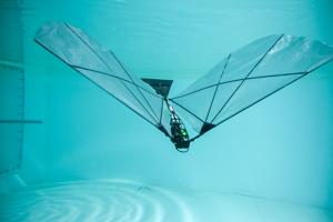
Physical robot

To verify that the conclusions drawn from the simulated robot can be extrapolated to the physical world, we built a robot with the same three-segment structure (Fig. 9a). We varied the amplitude of each of the two body joints at a constant frequency of 0.5 Hz.

Fig. 9: Locomotion of the physical robot. The alternative text for this image may have been generated using AI. Full size image a Top view image of robot with scale bar 35 mm. b Plot of angle vs. time inputs to the three motors during one cycle of the base gait. c Time series images of the robot using the base gait for half of one gait cycle at timesteps corresponding with the annotated plot of control signals. d Comparison of the speed of the physical robot and the simulated robot, varying the amplitude of the head joint (θ 2 ) oscillation. We held the other gait parameters constant, matching those tracked from P. senegalus: ϕ 2 = π/2, ϕ 3 = π, and A 3 = 2.1. e Comparison of the speed of the physical robot and the simulated robot, varying the amplitude of the tail joint (θ 3 ) oscillation. We held the other gait parameters constant, matching those tracked from P. senegalus: ϕ 2 = π/2, ϕ 3 = π, and A 2 = 1.5. f Comparison of the speed of the robot on different surfaces. “Base” denotes the robot with high friction fins on the low friction surface (µ s = 0.30), but the robot was not able to walk with the high friction fins on the high friction surface (µ s = 0.38). “Low fr fin” denotes the robot with low friction fins on the low friction surface (µ s = 0.27), and “high fr surface” denotes the robot with low friction fins on the high friction surface (µ s = 0.32). Error bars denote the standard deviation above and below the mean point for n = 5 trials.

Unlike in simulation, the potential for self-collisions between the rigid segments created kinematic constraints limiting the maximum amplitude of the head joint to θ 2 = 1.5 and the maximum amplitude of the tail joint to θ 3 = 2.1 (see “Methods” for more details).

Here, we found that the robot successfully moved forward (Supplementary Movie 6) and, like with the simulated robot, had the highest speed when moving with the gait parameters observed in P. senegalus. When varying the amplitude of the input to the head joint, the speed increased up to the maximum amplitude defined by its geometry (Fig. 9d). However, changing the amplitude did not change the speed of the physical robot as much as it changed the speed of the simulated robot. When varying the amplitude of the tail joint, the speed of the physical robot also increased as amplitude increased (Fig. 9e). The trajectory of the robot was consistent when keeping gait parameters constant (Supplementary Fig. 6), though the speed of the physical robot was much lower than the simulated robot until the highest amplitudes tested.