
Two families of multi-planet systems with distinct architectures and stellar hosts
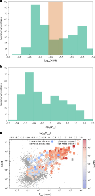
All queries filtered out systems with controversial planets, binary stellar systems and circumbinary planets to avoid biases due to the effects of the stellar companion. For each planetary system, we generated 105 synthetic copies where we randomly extracted the planetary and stellar parameters. 20), the orbital spacing metric S s (ref. We tested the hypothesis that the two families come from the same underlying distribution in terms of planetary architectures and stellar hosts by performing a two-sample KS test on all metrics: S m , S s , P out , N, NAMD and stellar properties: M * , [Fe/H], and PBM. We performed the two-sample statistical test (either KS or Wilcoxon–Mann–Whitney) for S s , S m , [Fe/H], P out , PBM, NAMD, M ⋆ and N on these two populations.
The sample of multi-planet systems and their host stars
We collected planetary data from the NASA Exoplanet Archive24 (https://exoplanetarchive.ipac.caltech.edu/) on 14 October 2025 using ExoplAn3T (Exoplanet Analysis and 3D Visualization Tool36, https://tools.ssdc.asi.it/exoplanet/) developed by the Space Science Data Center of the Italian Space Agency. ExoplAn3T allows searches based on the characteristics of planetary systems instead of individual exoplanets and has been used in previous studies focused on global investigations of exoplanetary systems3,4. We selected the sample of multi-planet systems through a two-step procedure. The first step involves a planetary query to identify exoplanets matching a specified set of characteristics, while the second step performs a system-wide query to retrieve data about all their planetary companions and their host stars. The data collected for sample L through the planetary and system-wide queries were filtered to preserve only multi-planet systems for which measurements and uncertainties on planetary mass (here both M p and \({M}_{{\rm{p}}}\,\sin \,i_{{\rm{p}}}\)) and semimajor axis were available for all planets. Sample H was derived by cross-matching sample L with the catalogue of stars for which we have homogeneous stellar parameters, as discussed in the following. For samples E and S, we included further filters on the orbital eccentricities and the planetary mass (here M p exclusively), respectively, and their uncertainties. All queries filtered out systems with controversial planets, binary stellar systems and circumbinary planets to avoid biases due to the effects of the stellar companion.
In the format of the NASA Exoplanet Archive24, the combined planetary and system queries for sample L are as follows:
default_flag = 1
sy_snum = 1
sy_pnum > 1
cb_flag = 0
pl_controv_flag = 0
pl_orbsmax not null
pl_orbsmaxlim = 0
pl_orbsmaxerr1 not null
pl_orbsmaxerr2 not null
pl_bmassj not null
pl_bmassjlim = 0
pl_bmassjerr1 not null
pl_bmassjerr2 not null
with the query for sample E adding:
pl_orbeccen not null
pl_orbeccenlim = 0
and that for sample S including also:
pl_massj not null
pl_massjlim = 0
pl_massjerr1 not null
pl_massjerr2 not null
During the computation of the global parameters of samples E and S, we also filtered out those systems containing planets for which the orbit was reported as non-circular but for which no uncertainty estimate was provided for the orbital eccentricity (only planets on circular orbits can have no uncertainty reported).
For each exoplanet, we retrieved the following parameters:
Host star name
Planet letter
Planet name
System multiplicity
Planetary orbital eccentricity and associated uncertainties
Planetary mass (in Jupiter masses) and associated uncertainties
Orbital semimajor axis of the planet and associated uncertainties
Planetary orbital inclination and associated uncertainties
HD name of the star
HIP name of the star
Right ascension of the star
Declination of the star
Gaia IDs of the star
The creation of sample H from sample L required that we derive homogeneous stellar data, which allowed us to more robustly test correlations and trends between planets and their host stars (for example, refs. 25,29,31,32,37,38,39,40). We cross-matched the multi-planet systems in sample L with the SWEET-Cat catalogue17,18 (http://sweetcat.iastro.pt), and we selected those stars that have been homogeneously characterized. This means that the effective stellar temperature T eff , metallicity [Fe/H] and surface gravity \(\mathrm{log}\,g\) have been determined with the same technique from high-resolution, high signal-to-noise spectra. The planet and host stars of sample H have temperatures 3,200 K ≤ T eff ≤ 6,600 K, metallicity −0.64 dex ≤ [Fe/H] ≤ 0.48 dex and surface gravity 2.6 dex \(\le \mathrm{log}\,g\le\) 5.1 dex.
We computed the stellar masses using the optimization tool PARAM (ref. 41,42,43), which we used to fit isochrones by comparing a grid of theoretical stellar isochrones with a set of observables, such as metallicity, effective temperature and photometric luminosity. The input luminosity L was computed separately by converting the bolometric magnitude M bol through the standard formula:
$$L=1{0}^{{M}_{\mathrm{bol}}}=1{0}^{-0.4\left(m+{\mathrm{BC}}_{m}-\left(-5+5\mathrm{log}(d)\right)-{M}_{\mathrm{bol},\odot }-{A}_{{\rm{m}}}\right)},$$ (1)
where m is the generic magnitude, BC m is its bolometric correction, d is the distance (in parsecs), M bol,⊙ is the bolometric magnitude of the Sun (4.74) and A m is the extinction for the m-band. M bol was derived from a Markov chain Monte Carlo fitting procedure, which took as input a combination of several magnitudes and their respective uncertainties. The magnitudes were taken from 2MASS44 (J-, H- and K s -bands), Gaia45 (G BP and G RP ) and when available, Johnson B and V magnitudes. The Johnson magnitudes were taken either from the synthetic photometry generated from Gaia BP/RP mean spectra46 or from the Tycho-2 catalogue (derived from the Tycho-2 B T and V T magnitudes)47, and we prioritized the first source. The distance was derived by a simple parallax inversion, with the parallax given by Gaia eDR3. The bolometric corrections were calculated using YBC48, which interpolates a series of precomputed tables for the bolometric correction with respect to T eff , [Fe/H], \(\mathrm{log}\,g\) and A V . For the theoretical models (the isochrones), we relied on PARSEC v2.1 (Padova and Trieste Stellar Evolution Code49, http://stev.oapd.inaf.it/cgi-bin/cmd).
Treatment of the missing eccentricities and inclinations in samples L, E and S
The query to create sample L (and, consequently, H) returns systems where the orbital eccentricity and inclination values are not known for all planets. To fill these gaps and compute the NAMD of these systems, we took advantage of the trends derived from the population of transiting planets characterized by the Kepler mission to fill the gaps with physically justified values. Specifically, we adopted the trends based on the criterion for the stability of the angular momentum deficit12:
$${\mu }_{{\rm{i}},{\rm{n}}}=1.1{0}_{-0.11}^{+0.15}\times {\left(\frac{N}{5}\right)}^{-1.7{3}_{-0.08}^{+0.09}}\,{\scriptstyle{\circ}\atop},$$ (2)
for the average multiplicity-dependent inclination and
$${\mu }_{e,n}=0.03{1}_{-0.003}^{+0.004}\times {\left(\frac{N}{5}\right)}^{-1.7{4}_{-0.07}^{+0.11}}$$ (3)
for the average multiplicity-dependent eccentricity. Rewriting these trends in the general form y = a × Cb where C = N/5 is a constant factor for each planetary system, the 1σ relative variability is \({\sigma }_{\mathrm{rel},y}\) \(=\sqrt{{({\sigma }_{a}/a)}^{2}+{(\mathrm{ln}(C){\sigma }_{b})}^{2}}\). The eccentricity and inclination of the individual planets in each system were computed assuming Gaussian distributions truncated to 0, centred on the average values set by μ e,n and μ i,n , and with the standard deviation associated with the relevant relative uncertainty σ rel,y . The queries to create samples E and S include, instead, systems where the inclination values are not known for all planets. To compute the NAMD of these systems, we took advantage of the knowledge of the orbital eccentricity, as it is known by definition for these samples, and assumed the Gaussian distributions of inclination centred on 0 with standard deviations equal to the modulus of the arcsin of the eccentricity \({\sigma }_{{\rm{i}}}=| \arcsin \,e|\) (ref. 4). This relation arises from the equipartition of the dynamical excitation \(\sqrt{{e}^{2}+{\sin }^{2}\left(i\right)}\) (ref. 50) along all secular degrees of freedom of the system2.
Normalized parameters and uncertainty propagation
To generate the Monte Carlo samples and quantify the uncertainties of the normalized parameters used in the analysis, we followed the Monte Carlo approach introduced by ref. 2 and updated in ref. 4. For each planetary system, we generated 105 synthetic copies where we randomly extracted the planetary and stellar parameters. Unless otherwise stated, we assumed for all planetary and stellar quantities Gaussian distributions truncated to 0 and centred on the nominal values, with standard deviations equal to half the full 1σ, 68% confidence interval. We quantified the nominal values and 1σ uncertainties of all normalized parameters from the modal values and the 16th and 84th percentiles of their posterior Monte Carlo distributions.
The normalized parameters adopted to quantify the basic physical properties of the multi-planet systems in the sample are the normalized planetary system mass NSM11,15 and the orbital period of the outermost planet P out , by analogy with the classical mass–period classification. The NSM metric is defined as
$$\mathrm{NSM}={{\Sigma }}_{i}{m}_{i}/{M}_{* },$$ (4)
where m i are the planetary masses, M ⋆ is the mass of the host star and the index i ranges from 1 to the planetary multiplicity N of the system. The nominal mass of the host star is that resulting from fitting the isochrone. The P out metric is defined as
$${P}_{\mathrm{out}}=\sqrt{\max {({a}_{i})}^{3}/{M}_{* }}\,\mathrm{years},$$ (5)
where the planetary semimajor axes a i are in astronomical units and M ⋆ is in solar masses. The normalized parameters used to characterize the global architecture of the planetary systems in the sample are the planetary multiplicity N (ref. 20), the fraction of the total planetary mass contained in the most massive planet S m (ref. 20), the orbital spacing metric S s (ref. 20) and the normalized angular momentum deficit NAMD (refs. 4,19,20) quantifying the dynamical excitation. In this study, we consider the planetary multiplicity N to be the number of known planets in each system, meaning that N > 1 by definition, as we focus on multi-planet systems. The mass partition S m metric is defined as
$${S}_{{\rm{m}}}={m}_{\mathrm{mp}}/{{\Sigma }}_{i}{m}_{i},$$ (6)
where m mp is the mass of the most massive planet. The orbital spacing metric S s is defined as
$${S}_{{\rm{s}}}=\frac{6}{N-1}\left(\frac{{a}_{\max }-{a}_{\min }}{{a}_{\max }+{a}_{\min }}\right){\left(\frac{3{M}_{* }}{2\overline{m}}\right)}^{1/4},$$ (7)
where \(\overline{m}={\Sigma }_{i}{m}_{i}/N\) is the mean mass of the planets, and a max and a min are the largest and shortest semimajor axes of the planets in the system. As discussed by ref. 20, this metric is also connected to the stability of multi-planet systems. Finally, NAMD is defined as
$$\mathrm{NAMD}=\frac{{\sum }_{i}{m}_{i}\sqrt{{a}_{i}}\left(1-\sqrt{1-{e}_{i}^{2}}\cos \,{i}_{i}\right)}{{\sum }_{i}{m}_{i}\sqrt{{a}_{i}}},$$ (8)
where e i and i i are the orbital eccentricity and inclination values of the planets, respectively. Following refs. 4,19,26, we adopted the NAMD of the Solar System4 (1.27 × 10⁻³) as the reference value for the transition between dynamical order and chaotic evolution (see refs. 2,51,52 and references therein).
For the masses of planets and stars we reused the values generated in the computation of NSM and S m . The shortest semimajor axis a min is the semimajor axis of the innermost planet for each synthetic planetary system. The values of a max were computed from the 105 Monte Carlo values of P out by inverting equation (5).
For the NAMD, we adopted the methodology from ref. 2 as expanded by ref. 4. We reused the 105 Monte Carlo extractions of the planetary masses m i and the semimajor axes a i described above and integrated them with 105 Monte Carlo extractions of the eccentricity and inclination values of all planets in the system. For those systems for which we possess inclinations for all planets, we assumed Gaussian distributions centred on the relative inclinations with respect to the most massive planet in the system and standard deviations equal to half the reported 68% confidence intervals2,3,26. For the systems for which we lack the eccentricity or inclination values of some planets, we followed the different approaches described in ‘Treatment of the missing eccentricities and inclinations in samples L, E and S’ for samples L and H and for samples E and S. For the systems in samples E and S for which we know the eccentricities of all planets, we followed the approach described by ref. 2 and assumed Gaussian distributions for the rectangular eccentricity coordinates \(\left(e\,\cos \,\omega ,\,e\,\sin \,\omega \right)\) where ω is the argument of periapsis. As the average value of ω did not influence the computation of the eccentricity distribution, its value was set to ω = 0 (ref. 2). The distribution of the first rectangular eccentricity coordinate \(\tilde{e}=e\,\cos \,\omega\) is therefore centred on the mean value 〈e〉 of the eccentricity, and the distribution of second rectangular eccentricity coordinate \(e\,\sin \,\omega\) is centred on 0. The standard deviations of both distributions were set to half the reported 68% eccentricity confidence interval. The distribution of e was derived from that of \(\tilde{e}\) through the relation \(e=\sqrt{{\tilde{e}}^{2}+{\left(\tilde{e}-\langle e\rangle \right)}^{2}}\) (ref. 2). In rare cases where the resulting value of e was outside the valid range [0:1), we repeated the Monte Carlo extraction of \(\tilde{e}\).
The normalized parameters used to characterize the host stars are the stellar metallicity [Fe/H], the stellar mass M * and the total PBM. For M * , we reused the 105 Monte Carlo values extracted for the computation of the NSM. For [Fe/H], we used the nominal values and uncertainties reported by SWEET-Cat. We used the synthetic values of stellar mass and metallicity to quantify PBM:
$$\mathrm{PBM}=\alpha +\beta \,{\mathrm{log}}_{10}({M}_{* })+[\mathrm{Fe}/{\rm{H}}]\,\mathrm{dex}.$$ (9)
This dependence of PBM on the parameters of the host star is based on the joint insights provided by the study of protoplanetary disks and of star–planet correlations. The first two terms on the right-hand side of equation (2) arise from the relation between the stellar mass and the dust mass in protoplanetary disks found by recent surveys21,22, with α and β being the fit parameters of this empirical correlation. In our analysis, we adopted the values α = 1.1 ± 0.2 and β = 1.9 ± 0.4 computed for the 1–2-Myr-old star-forming region L1688 by ref. 22. We extracted the 105 synthetic values of α and β from Gaussian distributions centred on the nominal values and with standard deviations equal to the uncertainties reported by ref. 22. We verified with numerical experiments that the specific choice of the star-forming region adopted as a reference did not affect the analysis, as its effect was simply to shift the absolute values of the PBM of the multi-planet systems. The second term in the right-hand side of equation (2) links the abundance of solid material in protoplanetary disks to the metallicity of their stars. The stellar metallicity is a proxy for the total abundance of heavy elements that can condense as solids in protoplanetary disks, and recent studies of the impact of stellar properties on planet formation highlight its important role in shaping the frequency and mass of planets (for example, refs. 25,29,30,31 and references therein).
Binning methodology
Owing to the large differences in the populations of the four samples, to plot the distributions of the normalized parameters in a uniform way we adopted for the optimal number of bins k in each plot the minimum between the values provided by Sturge’s formula (k = log 2 (n) + 1), the Rice rule (\(k=2\sqrt[3]{n}\)) and the Terrell–Scott rule (\(k=\sqrt[3]{2n}\)), after rounding to their least greater integers, where n is the total number of systems in the plot. Depending on the specific plot, therefore, n is either the total population of the sample or the combined population of lower-mass and high-mass systems, i.e. excluding the systems with uncertain attribution.
Statistical characterization of the two families and their properties
We identified the lower- and high-mass families by investigating the sample of multi-planet systems in the P out –NSM parameter space. We first analysed the distribution of each parameter individually using one-sample KS tests with the ks.test algorithm in the dgof package (https://www.rdocumentation.org/packages/dgof/versions/1.5.1/topics/ks.test) to test whether both NSM and P out are either normally or uniformly distributed. The comparison of both distributions provided P values much lower than 0.05 (Supplementary Table 3, top section) and rejected the hypothesis that either P out or NSM are normally or uniformly distributed. We then focused exclusively on the NSM metric and fitted a bimodal distribution to its values using a Gaussian mixture model implemented via GaussianMixture in the Python sklearn.mixture package53. We used a model with two components and max_iteration = 1,000 points, and we filtered out the systems from the sample that fell in the region where the two Gaussian components had comparable probabilities. We report in Supplementary Table 2 the number of systems U sys falling within this range, which we label as the ‘uncertain membership region’.
We then performed a statistical comparison between the two families of systems: the one with lower-mass architectures and the one with high-mass architectures (Fig. 1 and main text). These families were defined by the limits given by the Gaussian mixture fit of the NSM. We tested the hypothesis that the two families come from the same underlying distribution in terms of planetary architectures and stellar hosts by performing a two-sample KS test on all metrics: S m , S s , P out , N, NAMD and stellar properties: M * , [Fe/H], and PBM. We applied multiple testing corrections to the two-sample KS test results using the Holm–Bonferroni procedure, which controls the family-wise error rate in a stepwise manner while retaining the diagnostic power of the stricter Bonferroni method, yet without the same high rejection rate of true results. We also used the B-H procedure, which controls the false discovery rate under independence or certain forms of positive dependence among tests. For sample L, all results reported P < 0.05 (Supplementary Table 3), thus robustly supporting that the two families have intrinsically different properties. We repeated the same analysis on the H, E and S samples, whose P values always proved significant. The largest P values among all the metrics were 1.330 × 10⁻³ for the H sample (multiplicity N), 1.325 × 10⁻² for the S sample (PBM metric) and finally 2.061 × 10⁻² for the E sample (multiplicity N). When any of the presented metrics contained ties, we avoided the KS test, as it can yield inaccurate P values in such cases. Instead, we applied the non-parametric two-sample Wilcoxon–Mann–Whitney test by introducing an infinitesimal jitter (10−10) to both distributions to break the ties. The test was implemented using wilcox.test from the stats package in R54,55 (https://www.rdocumentation.org/packages/stats/versions/3.6.2/topics/wilcox.test).
Next, we tested whether the bimodality is a function of the stellar evolutionary phase using the H sample. Among the 189 multi-planet systems, 87.3% have main sequence stars. In this sample, only one lower-mass system has an evolved host star, whereas the high-mass family contains 23 evolved stars (Supplementary Fig. 2). Given that most of our sample are main sequence stars, we performed our tests on the main sequence subsample alone by conservatively removing all stars with \(\mathrm{log}\,g < 4\) from both lower- and high-mass families. This subsample includes 90 high-mass systems and 67 lower-mass systems around main sequence host stars. We note that both subsamples cover stellar spectral types from M to A. We performed the two-sample statistical test (either KS or Wilcoxon–Mann–Whitney) for S s , S m , [Fe/H], P out , PBM, NAMD, M ⋆ and N on these two populations. Each test (Holm–Bonferroni or B-H) resulted in P < 0.05 (the largest P value being 4.125 × 10⁻³ for N from the B-H correction), showing that the bimodality did not depend on the evolutionary stage of the host stars.
Finally, we used a Monte Carlo-resampled AD statistical pipeline to verify whether the different properties of the lower- and high-mass systems could have arisen from the uncertainties on the planetary and stellar parameters while simultaneously controlling for the false positive risks inherent in multidimensional parameter spaces. For the parameters spanning several orders of magnitude (NAMD, NSM and P out ), we applied logarithmic transformations (log 10 ) to the values, as in the distributions shown in Figs. 1 and 3. To account for measurement uncertainties, we modelled the probability density function of each parameter for each individual system using a Monte Carlo approach. For parameters with symmetric uncertainties, we generated 10,000 synthetic realizations drawn from a standard Gaussian distribution. For parameters exhibiting asymmetric uncertainties (for example, NAMD), we used split-normal distributions, randomly drawing 10,000 samples weighted by the independent upper and lower 1σ error boundaries. All distributions were truncated to 0 whenever necessary to prevent unphysical results. Deterministic parameters with no reported uncertainties (the planetary multiplicity N) were treated as static delta functions.
To determine whether the high- and lower-mass systems were drawn from the same underlying parent population, we employed the non-parametric k-sample AD test56 using the scipy.stats module within the SciPy module57 for scientific computing in Python. We independently executed the AD test on all 10,000 synthetic sets of parameters for the two families, yielding a distribution of P values. We extracted the 95th percentile of this P value distribution and considered each parameter to be provisionally distinct if this upper-bound P value fell below the standard significance threshold (P < 0.05). We verified the mathematical stability of this threshold by calculating the running 95th percentile across the iterations, ensuring all parameters reached asymptotic convergence well before the 10,000 iterations limit. Because we simultaneously tested nine physically coupled architectural parameters, we corrected for the probability of obtaining a spurious P < 0.05 result due to random chance (type I error) by subjecting the 95th percentile P values to the B-H procedure58. We classified a parameter as fundamentally distinct between the two populations only if its B-H-adjusted 95th percentile Monte Carlo P value remained <0.05. We applied this Monte Carlo-resampled AD procedure to all samples and verified that the two families always remain statistically different: the resulting distributions and the associated P values are reported in Extended Data Figs. 4–7. Because the scipy.stats.anderson_ksamp function hard caps its lowest possible reported P value at 0.001, when the output of the AD test corrected for the false discovery rate fell at this lowest bound, it is reported as p FDR < 0.001 in the plots.
Dynamical simulations of the possible origins of the excited architectures in the sample
Our exploratory campaign of instability simulations focused on investigating to what extent the dynamical excitation of the sample can inform us about the nature of the dynamical instabilities that caused it, that is whether they originated internally or externally to the planetary systems. Thus, we simulated the dynamical evolution of hundreds of synthetic planetary systems, sampling plausible initial architectures for both the lower- and high-mass families, and compared their final NAMD values with those of the real systems in samples L and E.
The synthetic lower- and high-mass planetary systems were described by the following common properties:
High-mass systems: P out = 5.25 years and NSM = 560 M ⊕
Lower-mass systems: P out = 0.1 years = 36.5 days and NSM = 33 M ⊕
Host stars: solar mass and radius (the latter quantity being used to test the possibility of stellar engulfments)
These properties position the lower-mass synthetic systems near the abundance peaks of their real counterparts in Fig. 1a,b. For high-mass synthetic systems, as NSM values close to the modal peak of the high-mass family proved extremely prone to becoming immediately unstable even when placed in resonant configurations, we focused the simulations on a lower NSM value. We adopted the following initial orbital architectures for both the lower- and high-mass synthetic systems:
(1) An initially unstable non-resonant configuration (at least one planet in the system is closer to the nearest planetary companion than the critical separation for stability59) (2) An incomplete resonant chain, such that the outermost planet is slightly shifted outwards with respect to the orbit that would result in a full resonant chain (3) Stable non-resonant configurations perturbed by the passage of a stellar intruder (all neighbouring pairs of planets in the system are more distant than the critical separation for stability59) (4) A stable resonant chain perturbed by the passage of a stellar intruder
As the instability simulations were solely focused on exploring the most probable instability trigger for lower- and high-mass systems, we adopted equal-mass planets as the reference set-up for all four initial orbital architectures. This choice was motivated by the observation that this initial state is compatible with systems belonging to both families (Fig. 2b and Extended Data Figs. 1–3). For scenarios 2 and 4, we focused on the 2:1 resonance after we verified with numerical experiments that it guarantees the highest initial stability for both lower- and high-mass systems.
To explore the impact of different mass partitionings among the planets, for scenario 4 we also considered the mass partition of the outer Solar System, that is 70% of the planetary mass is in the most massive object. This choice is again motivated by the observation that this initial state is compatible with systems belonging to both families (Fig. 2b and Extended Data Figs. 1–3). This choice also allowed us to take advantage of the extensive literature on the dynamical history of the Solar System and use one of its proposed initial architectures as a template for our synthetic lower- and high-mass systems (scenario 4-ss). Specifically, we followed refs. 28,52 and adopted the initial resonant five-planet configuration from ref. 60, which involves a mixed 2:1 and 3:2 resonant chain with another now-lost ice giant planet, and we scaled the planetary masses and the orbital period of the outermost planet to fit the requirements set for the synthetic lower- and high-mass systems28. For each architecture (scenarios 1–4 and 4-ss), we ran 100 instability simulations.
With the exception of scenario 4-ss, for which the initial number of planets was always set to 5, we randomly extracted the initial planetary multiplicity from a uniform distribution between 3 and 6. This choice was motivated by the observed NAMD–multiplicity anticorrelation among multi-planet systems4,19,26, which suggests that highly dynamically excited systems could have originally possessed more planets, as also illustrated by the dynamical studies by refs. 27,28. In scenarios 2, 4 and 4-ss, as the resonances set the spacing between the involved planets, we randomly varied the orbital angles to start the planets in different initial conditions. The stellar encounters that perturbed the stable systems in scenarios 3 and 4 were taken from the simulations of refs. 28,52. The time step of all simulations was set to 5% of the orbital period of the innermost planet. All instability simulations were run for 10 Myr, and we recorded all planetary collisions, ejections or impacts on the host star. At the end of the simulations, we characterized the outcomes in terms of the NAMD of the final planetary architecture, which we compare with the NAMD values of the real planetary systems in Fig. 3 and Extended Data Fig. 2 and with the number of planets lost through any of the previous processes. The results of this comparison are shown in Fig. 5.






© All Rights Reserved.