The planktonic microbiome of the Great Barrier Reef

Sample collection

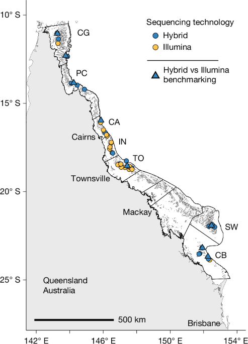
Samples were collected under the permit G12/35236–1 issued by the Great Barrier Reef Marine Park Authority. Seawater samples were collected from 48 coral reefs spanning the length of the GBR, aligning with in situ coral surveys by the AIMS LTMP in 2019 and 2020 (Fig. 1). Four 5-l biological replicates of seawater were collected above the reef (2–10 m depth) at each site (total n = 192) in either Nalgene or Niskin bottles and placed on ice until return to the vessel. Each 5 l volume was independently filtered successively through 5-µm, 33 mm diameter cellulose acetate and 0.22-µm Sterivex-GP filters (Millipore). The Sterivex filters were then snap frozen and stored at −75 °C until DNA extraction.

In addition to metagenomics data, a total of 17 physicochemical variables were measured as part of this survey on 3 of the 4 replicates (5 l each) from each site, including ammonia (NH 4 +), nitrite (NO 2 −), nitrate (NO 3 −), total dissolved nitrogen, phosphate (PO 4 3−), total dissolved phosphorus, dissolved organic carbon, silicate, total suspended solids, chlorophyll a pigment concentration, phaeophytin A, particulate organic carbon, particulate nitrogen, particulate phosphorus, temperature, salinity and chlorophyll a fluorescence, using methods described in Terzin et al.76.

DNA extraction

DNA extractions were carried out inside each 0.22-µm Sterivex filter by adding 1.8 ml filter-sterilized lysis buffer containing 50 mM Tris-HCL (pH 8.0), 40 mM EDTA (pH 8.0), 256 mg ml−1 sucrose and 18 µl lysozyme (100 mg ml−1). The filters were incubated with mild agitation for 1 h at 37 °C, followed by the addition of 20 µl proteinase K (20 mg ml−1) and further incubation and agitation for 1 h at 55 °C. The lysate was then ejected through the Sterivex into a 5 ml microtube and an equal volume of phenol:chloroform:isoamyl alcohol (IAA; 25:24:1) was added, mixed by inversion and centrifuged at 16,000g for 10 min. The aqueous phase was then recovered and an equal volume of chloroform:IAA (24:1) was added and mixed by inversion, then centrifuged for 10 min at 16,000g. DNA was precipitated by adding 1 ml isopropanol and recovered by centrifugation at 20,000g for 25 min and the supernatant discarded. The DNA was washed with 500 µl 70% ethanol, centrifuged for 10 min, the ethanol discarded and the pellet air-dried. Finally, 20 µl PCR water was added, incubated at 4 °C overnight to resuspend the DNA pellet and frozen at −20 °C.

Illumina sequencing

All 191 replicates from the 48 sites were subjected to Illumina sequencing at the Centre for Microbiome Research (Brisbane, Australia). Libraries were prepared using the Nextera DNA Flex Library Preparation Kit (Illumina 20018705) according to manufacturer’s protocol. Libraries were pooled at equimolar amounts of 2 nM per library. The library pool was quantified in triplicates using a Qubit dsDNA HS Assay Kit (Invitrogen) and sequenced using an S4 2× 150 bp flow cell on a NovaSeq 6000. Additional ‘deep’ sequencing was carried out for one replicate from 27 of the 48 sites to a target depth of 40 Gbp for Nanopore polishing and hybrid assembly (Supplementary Tables 1 and 2).

Nanopore sequencing, basecalling and quality control

The replicate chosen for Illumina deep sequencing was also submitted for long-read sequencing on Oxford Nanopore Technology’s (ONT) PromethION platform at the Australian Centre for Ecogenomics (Brisbane, Australia) sequencing facility. For ONT sequencing, DNA was first size-selected using the Circulomics SRE XS kit (PacBio, SKU 102-208-200) as this was shown in a small trial to increase total data output and read N50. Native barcoded libraries were prepared from the size-selected DNA following a genomic DNA by ligation protocol (Oxford Nanopore, LSK-109 with EXP-NBD104). Barcoded libraries were pooled with two samples per PromethION flow cell at equal concentration and the library pool was sequenced on a PromethION 24 (Oxford Nanopore) for a total of 72 h with a R9.4 flow cell using MinKNOW (v20.06.18) with default settings. We then performed rebasecalling of the fast5 files using the superaccuracy model with Guppy (v5.0.16) to generate higher accuracy raw reads before assembly. Finally, Porechop (https://github.com/rrwick/Porechop; v0.2.4) was used for barcode trimming using default settings.

Hybrid metagenome assembly

Deep Illumina and nanopore reads for each of the 27 sites were assembled using the Aviary assembly pipeline (https://github.com/rhysnewell/aviary; v0.3.3), specifying the ont_HQ flag for long reads. In brief, by supplying both short and long reads for hybrid assembly, Aviary first assembled the nanopore reads with metaFlye77 (v2.9), then polished the metaFlye assembly using a series of Racon78 (v1.4.3; three rounds), Pilon79 (v1.23; one round), and Racon (one round). Next, a subset of high-coverage, polished metaFlye contigs were identified and Illumina reads from the same replicate were mapped to them. Illumina reads that did not map to these contigs were assembled using metaSPAdes80 (v3.15.3) together with the nanopore reads. Finally, the hybrid-assembled contigs were collated with the high coverage polished metaFlye contigs to produce the final assembly. For the remaining 21 sites not chosen for Nanopore sequencing, a single replicate was assembled using the Aviary pipeline which used metaSPAdes for Illumina-only assembly.

Prokaryote genome binning and analysis

Assemblies were binned using the Aviary pipeline’s recover workflow, which first mapped reads to each assembly using Minimap281 (v2.18). For differential coverage binning, three sites were chosen for mapping to each assembly based on geographical proximity and all nanopore and Illumina reads for all four replicates from each site were used (Supplementary Table 22). Aviary recover then ran binning programs MetaBAT82, MetaBAT 2 (ref. 83) (v2.15), MaxBin 2.0 (ref. 84) (v2.2.7), Rosella (https://github.com/rhysnewell/rosella; v0.3.3), CONCOCT85 (v1.1.0) and Vamb86 (v4.0.0) and included a bin refinement step through Rosella to further refine bins based on kmer frequency and coverage. Finally, Das Tool87 (v1.1.2) was used to collate a representative set of bins from across the different binning tools. pMAGs were retained if they passed a quality threshold ≥50 (quality = completeness − 3 × contamination) using either CheckM1 (ref. 88) (v1.2.1) or CheckM2 (ref. 89) (v1.0.2), such that pMAGs of lower completeness were allowed lower contamination scores for inclusion. Taxonomic classification of the pMAGs was performed using the Genome Taxonomy Database Toolkit90 (v2.3.0) with database release R214. Dereplication of MAGs for mapping, and for assessment of presence within previously published databases and data sets including the OMD4 and Australian National Reference Stations91, was carried out using CoverM92 cluster (v0.6) at 95% ANI. Relative abundance was calculated by mapping the Illumina reads to the dereplicated set of reference pMAGs using CoverM genome, requiring 95% identity and 75% read length alignment to consider a read mapped.

Benchmarking hybrid assembly MAG binning

To directly benchmark the effect of including long nanopore data on improving MAG recovery, we undertook separate re-assembly and binning of eight replicates spanning sites from north to south of the GBR. To remove the effect of sequencing depth, we compared two treatments: (1) Illumina-only assembly of 30 Gbp of sequence data using metaSPAdes; and (2) a separate assembly using a subset of 15 Gbp of Illumina reads combined with 15 Gbp of nanopore reads as described above for hybrid assembly. The resulting 16 assemblies were binned with Aviary recover to obtain pMAGs as described above. Genomic diversity of the recovered pMAGs was estimated with inStrain24 (v1.7.1) by mapping Illumina reads to their respective metagenome assemblies using Bowtie 2 (ref. 93) (v2.4.5) followed by CoverM filter to select mapped reads with at least 95% identity and 75% read alignment.

Microbial community composition and function

Read mapping counts to the 95% ANI dereplicated set of pMAGs and relative abundances generated using CoverM genome described above were used to visualize community composition and clustering through principal component analysis ordinations in R (ref. 94) (v4.4.1) using the vegan95 package (v2.6.8). Relative abundances were summarized to genus and other higher taxonomic ranks using phyloseq96 (v1.48.0). Associations between community composition, GBR sectors, and reef zoning were assessed using PERMANOVA implemented in vegan, while associations between pMAGs with NTMR and Fished reefs were assessed using generalized linear models implemented in MaAsLin 3 (ref. 97) (v0.99.4) controlling for variability across sectors and Benjamini–Hochberg false discovery rate correction for multiple comparisons. Figures showing maps of the GBR and zoning boundaries (for example, Fig. 1) were drawn in R using Geographic Information System data available in the gisaimsr (v0.0.1) R package (https://open-aims.github.io/gisaimsr/index.html).

To assess functional potential of microbial communities in IN and TO sectors, genes were first predicted from IN and TO metagenome assemblies using Pyrodigal98 (v3.7.0) followed by clustering at 95% identity using MMseqs2 (ref. 99) (v13.45111) to create a non-redundant gene catalogue. Trimmed sequence reads from each IN and TO metagenome were then mapped to this catalogue using CoverM make and read mapping counts subsequently calculated from the output bam files using Samtools100 (v1.21). Representative sequences in the non-redundant catalogue were assigned to Kyoto Encyclopedia of Genes and Genomes Orthology using KofamScan101 (v1.3.0). Differential abundance statistics on the read mapping counts from CoverM and Samtools were generated using DESeq2 (ref. 102) (v1.44) in R.

Bioindicators of reef zoning

To identify bioindicators of NTMR and Fished reefs, we first performed feature selection using MINT sPLS-DA103,104 implemented in mixOmics105 (v6.26.0) to account for sectors on the GBR, using centred log ratio-transformed abundances of the 95% ANI dereplicated set of 876 pMAGs, 362,802 vOTUs and 1,136,487 eukaryote contigs (see ‘Final GBR-MGD database compilation’). Random forest (ranger R package v0.17.0) was then used on the selected features to assess accuracy in predicting reef protection zones (average accuracy over 50 runs), using leave one group out cross validation to account for sectors on the GBR. This analysis was then repeated on pMAGs alone with the first MINT sPLS-DA component consisting of the top 60 selected indicator taxa. Differences in average genome size and GC content between indicators of NTMRs and Fished reefs were visualized as box plots using ggplot2 (v3.5.1), and the variation in genome size and GC content was compared between indicators of NTMRs and fished reefs with pairwise Wilcoxon rank-sum tests.

To identify environmental drivers that explained differences in indicator taxa between NTMR and Fished reefs, the 60 indicator pMAGs of reef zoning were correlated with each of the 17 physicochemical variables using MINT sPLS. sPLS106,107 models the relationship between multiple predictors (physicochemical variables) and multiple responses (microbial taxa), while MINT103 integrates samples from independent subsets to account for confounding effects, such as season and geography. Median values for each physicochemical variable were first calculated per reef site, as the number of replicates differed for molecular (n = 4) and water chemistry (n = 3) samples. We then correlated centred log ratio-transformed abundances of the 876 dereplicated pMAGs with the 17 physicochemical measurements. Similarity scores (partial correlations) were visualized in ggplot2 (v3.5.1). All analyses were implemented in R. Final composite plots were edited for clarity in Inkscape (v0.92.5).

Viral, plasmid and eukaryote contigs

The following viral prediction tools were used to identify putative viral contigs from the GBR-MGD metagenomic assemblies: GeNomad46 (v1.5.018; --enable-score-calibration --min-score=0.7 --max-score=0.1) with database v1.2, VirSorter2 (ref. 47) (v2.2.431; --include-groups “dsDNAphage,NCLDV,RNA,ssDNA,lavidaviridae”, --min-score=0.9) with database v1.2, ViralVerify108 (v1.133; -thr 7), VIBRANT109 (v1.2.132), PPR-Meta110 (v1.134; -t 0.9), and DeepVirFinder111 (not versioned; retrieved from GitHub on 8 March 2023; P value < 0.05). Putative viral contigs were then input into CheckV112 (v1.0.1) with database v1.5 for quality trimming and assessment. Viral predictions were examined using CheckV’s curated marker sets by visualizing the ratio of host:viral markers and the proportion of viral markers for each putative virus prediction to assess whether the contigs predicted by each tool were host- or virus-derived.

In addition to three viral prediction tools that also predicted plasmids (GeNomad, PPRMeta and ViralVerify), two additional plasmid-only prediction tools were used on the metagenomic assemblies, PlasForest113 (v1.2), and PlasX114 (unversioned; score ≥0.9), which uses annotated gene families generated in anvi’o115 (v7.1) using the COG2014 and Pfam v32 databases. Whokaryote116 (v1.1.2) and EukRep117 (v0.6.6) were used for eukaryotic prediction.

Manual curation of picoeukaryote genomes

Genomes of two picoeukaryotes from the Mamiellales family, Bathycoccus prasinos and Ostreococcus sp. clade B, were manually curated after initial blast results of partial eMAGs revealed the presence of potential Bathycoccus and Ostreococcus long contigs in high abundance as determined by read mapping. Therefore, complete genomes for the sequenced Mamiellales isolates B. prasinos RCC1105, Micromonas commoda RCC299, Micromonas pusilla CCMP1545, Ostreococcus lucimarinus CCE9901, Ostreococcus tauri and Ostreococcus spp. RCC809 were retrieved from the RefSeq database and used as references for competitive mapping of large metagenomic contigs (≥50 kb) with Minimap2 (ref. 81) (v2.28) using its genome/assembly alignment mode, allowing up to 20% sequence divergence (--asm20). The majority of contigs were recruited by either B. prasinos RCC1105 or Ostreococcus spp. RCC809, and were selected for manual curation of two distinct species using the RCC1105 and RCC809 genomes as references. Contigs recruited by Ostreococcus spp. RCC809 also showed high recruitment to O. lucimarinus CCE9901, which was therefore used as a secondary reference as needed. Contigs were aligned to the corresponding reference using progressiveMauve from the Mauve aligner118 (v2015-02-13). In the few cases where a chromosome was recovered in a sample fragmented in 2–4 contigs, Mauve Contig Mover from the Mauve program was used to reorder and link the chromosomal fragments with a linker of 100 Ns. Telomeres were identified at the ends of chromosomal contigs using Tidk119 (v0.2.65) to search for telomeric repeat sequence AACCCT, followed by visual inspection to confirm elevated numbers of telomeric repeats at the ends of contigs using Tidk plot.

Marine Crassvirales

vMAGs classified by GeNomad as Crassvirales were annotated using Pharokka120 (v1.6.1) with additional Crassvirales protein profiles provided by Yutin et al.59. To verify the GeNomad classifications, we downloaded the set of Caudoviricetes TerL sequences compiled by Piedade et al.62 and aligned TerL sequences detected in the vMAGs (>400 amino acid residues) to this collection using MAFFT121 (v7.508). The output sequence alignment was trimmed with trimAl122 (v1.4.rev15; -gt 0.2) and used to infer a bootstrapped phylogenetic tree using IQ-TREE 2 (ref. 123) (v2.2.0.3). Separately, we constructed a proteomic tree using the vMAGs (>20 kb) based on genome-wide sequence similarities computed using tBLASTx as implemented in ViPTree124 (v4.0). Both trees were visualized and edited for clarity in ITOL125 (v7) and Inkscape (v0.92.5). Host prediction was performed on vMAGs using iPHoP126 (v1.3.3) with the supplied Aug_2023_pub_rw database including pMAGs dereplicated at 99% ANI (using CoverM) added to this host database.

Final GBR-MGD database compilation

The GBR-MGD database is composed of prokaryotic MAGs, manually curated Mamiellales genomes, and contigs identified as plasmid, viral, or eukaryotic. A standardized labelling scheme with the structure of IMOS__<TaxaGroup>__SAMPLENAME__CONTIG:<TaxaComponent> was applied to all sequences. TaxaGroup indicates all taxa that were linked to that contig (E = eukaryote, M = plasmid/mobile element, P = prokaryote, V = virus). Contigs marked with only one group were only identified to belong in that group, while contigs marked with multiple letters indicate they were linked to more than one group. For example, a contig marked with a V indicates that the contig was identified as a virus but is not found in another group. PV indicates that a contig is present in a pMAG and predicted to be a virus or provirus, MPV indicates that a contig is found in a pMAG and predicted to be a plasmid and virus. As viruses can be predicted within other taxa (for example, PV contigs), TaxaComponent indicates the taxa represented by a particular sequence as well as the bp position in the case of some viral sequences. For example, a proviral region identified within a prokaryotic bin would be represented by two distinct sequences. The sequence within the prokaryotic bin would be labelled IMOS__PV__SAMPLE__CONTIG:p while its counterpart representing the viral prediction would be labelled IMOS__PV__SAMPLE__CONTIG:v1001-10000. Additionally, contigs are labelled with the prediction tools used to group them into their respective TaxaGroup.

The prokaryotic bins and manually curated Mamiellales genomes were dereplicated together using CoverM. Contig predictions were dereplicated separately for each taxon group (for example, V, P, E or PV) using pairwise ANI (95% ANI + 85% alignment fraction) using the anicalc.py and aniclust.py scripts provided by CheckV. Relative abundance of each component of the database was calculated by mapping the Illumina metagenomic reads to each taxon group in the final dereplicated database separately using CoverM Genome, requiring 95% identity and 75% alignment to be considered mapped.

Reporting summary

Further information on research design is available in the Nature Portfolio Reporting Summary linked to this article.