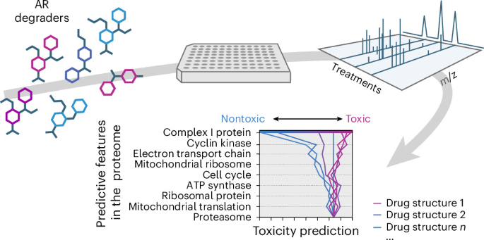
Proteome-guided drug discovery maps and mitigates therapeutic degrader toxicity

In vivo experimental design

The C4-2 xenograft study was carried out at Axis Bioservices in accordance with UK Home Office legislation and the Animal Scientific Procedures Act 1986. IVC-cage group-housed immunocompromised NOD-SCID male mice (Envigo; aged 5–8 weeks) were used for subcutaneous tumor implantation of C4-2 cells (1 × 107 cells 1:1 in Matrigel) using a 23-gauge needle. The animal holding room was maintained at room temperature (18–24 °C), humidity at 30–70% and a 12-h light–dark cycle. Mice were surgically castrated when tumors reached approximately 150 mm3 and dosing started 3 days later. Compound 3 was formulated with amorphous solid dispersion in 0.5% w/v HPMCAS and 0.5% w/v Methocel A4M in water pH 7.4 and orally dosed once daily (30 mg kg−1). Enzalutamide was formulated in 5% DMSO and 95% Methylcellulose (0.5% w/v) with 0.1% Tween-80 and orally dosed once daily (50 mg kg−1). The length (L) and width (W) of tumors were measured by bilateral Vernier caliper and tumor volume was calculated as (π × maximum measure (L or W) × minimum measure (L or W) × minimum measure (L or W))/6,000. TGI from the start of treatment was assessed by comparison of the geomean change in tumor volume for the control and treated groups. Statistical significance was evaluated using a one-sided t-test. All in vivo studies complied with all relevant ethical regulations for animal testing and research, followed AstraZeneca’s global bioethics policy and received ethical approval from the AstraZeneca ethical committee.

Xenograft sample preparation

Animals were killed and tumor samples were snap-frozen in liquid nitrogen for subsequent analysis. Tumor pieces were lysed in 1 ml of ice-cold buffer containing Tris-NaCl pH 7.5 20 mmol l−1, NaCl 137 mmol l−1, glycerol 10%, 1% SDS, 1% NP-40 substitute supplemented with NaF 50 mmol l−1, Na3VO4 1 mmol l−1, protease complete inhibitor tablet (Roche 1836145), benzonase nuclease 1 μl per 5 ml (Sigma-Aldrich E1014-5KU) and phosphatase inhibitor cocktails 2 and 3 (Sigma-Aldrich, P0044 and P5726). Homogenization was performed 3× using Fastprep tubes (MP Biomedicals, 6910-500) and an MP Biomedicals Fast Prep-24 machine. All samples were sonicated for 30 s at high amplitude (Diagenode). Samples were then centrifuged at 10,000g and 4 °C for 15 min and the supernatants were collected and stored at −70 °C before immunoblot analysis.

Xenograft immunoblotting

AR protein levels were assessed using standard western blotting techniques (NuPAGE Novex 4–12% Bis–Tris gels and iBlot nitrocellulose transfer stacks (Thermo Fisher, IB23001), with 7-min transfer at 20 V). Antibodies were diluted in 5% Marvel in TBS and 0.05% Tween-20 and the signal was detected using a SuperSignal West Dura horseradish peroxidase (HRP) substrate on a Syngene G Box. The AR antibody was purchased from Dako (M3562; 1:1,000). Quantification was carried out on nonsaturated images using the Syngene Genetools software with automatic background correction.

Human hepatocarcinoma HepG2 C3a cell culture

HepG2 C3a cells were sourced from AstraZeneca’s Global Cell Bank (American Type Culture Collection (ATCC), CRL-3581). Cells were cultured in DMEM (Thermo Fisher, 1196025) supplemented with 10% (v/v) FBS (Gibco, 10010056) and 10 mM glucose (Sigma, 16320, prepared as a sterile 50× stock) at 37 °C, 5% CO 2 . Cells were passaged at 80% confluency until at least 90% viability was obtained. Cells were counted using a Vi-CELL (Beckman Coulter, 383556) and diluted to 0.6 × 106 cells per ml in complete DMEM, such that dispensing 100 µl will result in 60,000 cells per well. The cell suspension was added to 96-well plates (Corning Costar, 3596) using a Multidrop Combi (Thermo Fisher, 5840300) with a standard-tube cassette (VWR, 735-0260). Cells were allowed to adhere 24 h before compound treatment, under normal growth conditions.

High-throughput screening of drug libraries on HepG2 cells

FDA-approved drug screening was performed using a premade library purchased from Selleck Chemicals (L1300). The library was reconstituted in DMSO and diluted 1:10 in distilled water to prepare 1 mM drug stocks. HepG2 cells in 96-well plates were then refreshed with 200 µl of growth medium using a liquid-handling robot (Biomek). For drug treatment, 20 µl of the respective stocks were dispensed into wells at a 1:100 dilution with automated handling to reach final concentrations of 10 µM. The treated samples were then incubated at 37 °C with 5% CO 2 constant (v/v) for another 24 h. For harvesting, samples were washed three times in 200 µl of PBS, aspirated and stored at −80 °C until further processing. HBD library screening was performed using compounds synthesized and sourced through the AstraZeneca Compound Management Group. Compounds were prepared as 0.1, 1 and 10 mM source stocks in DMSO. Medium was removed from the assay plates and 30 µl of fresh medium was added to each well using a Multidrop Combi with standard-tube cassette. An integrated robotic system from HighRes BioSolutions controlled by Cellario software (HighRes BioSolutions) was used to perform the assay. Assay plates were dosed using an Echo 655T acoustic dispenser (Labcyte) from the appropriate compound stock to perform at 1,000-fold dilution (final volume of 100 µl per well) resulting in assay concentrations of 0.1, 1 and 10 µM. Addition of medium to a final volume of 100 µl was performed using a Multidrop Combi. Assay plates were return to the SteriStore incubator for a further 24 h before cell harvesting. Cells were washed twice with PBS (Merck, D8662) using a Multidrop Combi with a standard-tube cassette. Plates were dried of all buffer and frozen at −80 °C until sample processing for proteomics.

Cell line immunoblotting

HepG2 (ATCC, CRL-3581) were grown in RPMI-1640 and DMEM Glutamax with 10% FBS (Thermo Fisher, 10270-106) for 24 h. The cells were then washed with PBS and harvested with RIPA containing protease inhibitor. The lysates were centrifugated for 10 min at 14,000g at 4 °C. The supernatants were collected and subjected to SDS–PAGE analysis using the Odyssey system. For the detection of the AR protein, the monoclonal mouse anti-human AR antibody from DAKO was used (M3562; 1:1,000).

LNCaP cells (ATCC, CRL-1740) were grown in RPMI-1640 with 8–10% FBS and 1% glutamine. Cells were treated with compound for 24 h and lysates were then harvested, sonicated and centrifuged (10 min, 14,000g at 4 °C). Protein content of supernatants was quantified using the BCA protein assay kit according to the manufacturer’s protocol. An equal amount of protein from each sample was subjected to SDS–PAGE analysis using NuPAGE 4–12% Bis–Tris Gels and iBlot nitrocellulose transfer stacks. Membranes were blocked in TBST with 5% nonfat dry milk and incubated with anti-AR (Dako, M3562; 1:1,000), anti-PSA (Cell Signaling Technologies, 5365S; 1:1,000) or anti-GAPDH (Cell Signaling Technologies, 5174, 1:1,000) antibodies, followed by HRP-conjugated antibodies. Signal was detected using SuperSignal WestDura (Pierce, 34075) on the ChemiGenius or Gbox (Syngene).

HepG2 glucose and galactose assay

The glucose and galactose assay aims to detect compound causing cytotoxicity in HepG2 cells cultured in medium containing either glucose or galactose. The assay uses the Promega CellTiter-Glo endpoint to measure cell viability on the basis of a luciferase reaction to determine the amount of ATP in viable cells. HepG2 cells grown in the presence of galactose instead of glucose in the medium increase oxygen consumption, which is indicative of a switch from glycolysis to mitochondrial-dependent oxidative phosphorylation. When the toxicity by mitochondrial toxins and drugs with known mitochondrial liabilities were compared under both culture conditions, cytotoxic effects were observed at lower concentrations in cells grown in galactose. Hepg2 cells were seeded in a 384-well plate in 95 µl of glucose or galactose medium at 5,000 cells per well. The cells were allowed to adhere overnight at 37 °C before adding 5 µl of compound to cells for 24 h. Then, 10 µl of Promega CellTiter-Glo was added per well for 20 min at room temperature before reading luminescence.

HepG2 mitochondrial respiration assay

The XFe96/XF Pro sensor cartridge (Agilent, 103793-100) was rehydrated with pure water in a CO 2 -free incubator at 37 °C overnight. Cells were seeded in XFe96/XF Pro cell culture microplates (Agilent, 103794-100). Cells were incubated with Seahorse XF DMEM assay medium (Agilent, 103680-100) supplemented with 10 mM glucose (Agilent, 103577-100), 1 mM pyruvate (Agilent, 103578-100) and 2 mM glutamine (Agilent, 103579-100) in a CO 2 -free incubator at 37 °C for at least 1 h before performing the assay. Water in the XFe96/XF Pro sensor cartridge was replaced with warm Seahorse XF calibrant solution (Agilent, 100840-000) and incubated in a CO 2 -free incubator at 37 °C for at least 45 min before performing the assay. Cells were dosed and mitochondrial function was measured with a Seahorse XF Pro Analyzer by Agilent and Seahorse XF cell mito stress test kit (Agilent, 103015-100). The protocol used consists of calibration and equilibration, basal respiration registered every 3 min ten times, injection of oligomycin 1.5 μM and OCR measurement every 3 min three times, injection of carbonylcyanide-p-trifluoromethoxyphenylhydrazone 1 μM and OCR measurement every 3 min three times and injection of rotenone + antimycin A 0.5 μM every 3 min three times. Afterward, cells were fixed in 4% paraformaldehyde (diluted in PBS; Sigma, P6148) for 10 min at room temperature. They were washed with PBS and incubated with Hoechst33342 at 1:5,000 (Invitrogen, H3570) for 10 min at room temperature. Cells were again washed and left in PBS for imaging with BioTek Cytation 5 cell-imaging multimode reader by Agilent. OCR measurements were normalized for the number of cells. OCR values registered after rotenone + antimycin A injection were used to define nonmitochondrial respiration. These values were subtracted from the OCR measurements of each sample. Data were normalized to the basal respiration of DMSO-treated samples.

Bovine heart complex I assay

Bovine heart mitochondria prepared using the protocol by Fedor and Hirst37 and membranes were prepared using the protocol by Blaza et al.38. Membranes were diluted to 25 µg ml−1 in membrane assay buffer (250 mM sucrose and 10 mM Tris-HCl pH 7.5 at 32 °C) and supplemented with 3 µM horse heart cytochrome c (Merck) and 200 µM NADH (Merck) to start complex I–III–IV turnover (NADH oxidation). NADH oxidation was monitored using difference absorbance (340–380 nm, extinction coefficient = 4.81 mM−1 cm−1) over 20 min. Compounds were added from 100-fold concentrated DMSO stocks, with 1% DMSO (v/v) included as a control. All measurements were made in triplicate at 32 °C in a 96-well Molecular Devices plate reader. Data were collected across three separate experiments.

Bovine heart complex II assay

Bovine heart mitochondrial membranes were diluted to 25 µg ml−1 in membrane assay buffer with 3 µM horse heart cytochrome c. The reaction was initiated by adding 5 mM succinate, 1 mM K 2 SO 4 , 2 mM MgSO 4 , 60 µg ml−1 fumarase (Escherichia coli FumC, purified in-house), 300 µg ml−1 oxaloacetate-decarboxylating malate dehydrogenase (E. coli Maeb, purified in-house) and 2 mM NADP+. Compounds were added from 100-fold concentrated DMSO stocks, with 1% DMSO (v/v) included as a control. NADP+ reduction was monitored using the difference in absorbance (340–380 nm, extinction coefficient = 4.81 mM−1 cm−1) over 20 min. All measurements were made at 32 °C in a 96-well Molecular Devices plate reader. Data were collected across three separate experiments.

Primary human hepatocyte survival assay

Transporter-certified donor lots of cryopreserved primary human hepatocytes were obtained from BioIVT. The donor lots used were WID and JEL. Williams E medium and Matrigel were obtained from Sigma-Aldrich (W1878-500ML). Hepatocyte plating (CM3000) and supplement (CM4000) packs were obtained from Thermo Fisher Scientific. Promega CellTiter-Glo luminescent cell viability assay and ApoTox-Glo triplex assay kits were obtained from Promega. Primary human hepatocytes were rapidly thawed in hepatocyte thawing and plating medium (Williams E medium supplemented with 5% FBS, 1 µM dexamethasone, 1% penicillin–streptomycin, 4 µg ml−1 human recombinant insulin, 2 mM GlutaMAX and 15 mM HEPES pH 7.4), pelleted at 100g for 10 min and resuspended in hepatocyte thawing and plating medium. The cells were pelleted at 100g for 5 min and resuspended a second time before cell number determination using trypan blue exclusion. The cells were then seeded at 70,000 cells per well in 125 µl per well into 96-well collagen-coated plates. All hepatocytes, after incubation at 37 °C in a humidified chamber for 4–6 h, were then overlaid with Matrigel (0.25 mg ml−1) in ice-cold hepatocyte culture medium to produce a ‘sandwich culture’ and then incubated for a further 18–20 h at 37 °C in a humidified chamber. Then, 24 h after seeding, the medium was removed from the wells and replaced with fresh culture medium (125 µl per well). Hepatocytes were dosed with compounds using the Tecan D300 at concentrations of 0, 0.25, 0.5, 1, 2.5, 5 or 10 µM with a final DMSO vehicle concentration of 0.2%. Hepatocytes were incubated for a further 24 h at 37 °C in a humidified chamber. ATP content was determined using the Promega CellTiter-Glo luminescent cell viability assay following the manufacturer’s protocol. Luminescence was determined on a Perkin Elmer Envision microplate reader.

Nanoluciferase degradation assay

Compound assay-ready plates were prepared using acoustic dispensing (Echo), generating 12-point, half-log dose responses with a top concentration of 30 µM. Wells were backfilled with DMSO to 0.3% DMSO. DMSO and pomalidomide (30 µM) were used as neutral (0) and 100% degradation (−100), defining the scale range. HiBiT–IKZF3 MM.1S cells and HiBiT–SALL4 SK-N-DZ cells were started from cryovials into their respective media and dispensed onto compound assay-ready plates at either 3,000 (SALL4) or 20,000 (Aiolos) cells per well using a Multidrop Combi. Plates were subsequently spun for 1 min at 300g and incubated for 6 h at 37 °C, 5% CO 2 in a humidified incubator. HiBiT lytic detection reagents (Promega) were prepared according to the manufacturer’s instructions and 5 µl per well of the lytic detection mix was added to each plate using a Multidrop Combi. Plates were spun for 1 min at 300g and placed on an orbital shaker at 3g for 30 min before reading luminescence on an Envision plate reader according to the manufacturer’s instructions.

HiBiT–IKZF3 MM.1S cells (obtained from Promega, CS3023229) were grown in RPMI-1640 (Gibco), supplemented with 10% FBS and GlutaMAX (Gibco). HiBiT–SALL4 SK-N-DZ cells (obtained from Promega, CS3023238) were grown in high-glucose DMEM (Gibco), supplemented with 10% FBS, GlutaMAX (Gibco), sodium pyruvate (1 mM) (Gibco) and 1% nonessential amino acids (Sigma).

Cancer cell line proliferation assays with analogs

To measure growth, LNCaP (ATCC, CRL-1740), VCaP (ATCC, CRL-2876), SU.86.86 (ATCC, CRL-1837) and Mia PaCa-2 (ATCC, CRL-1420) cells were seeded in 96-well plates and dosed with compounds 24 h later up to 30 µM. The number of live cells was determined at day 0 and days 5–8 (depending on the cell line) using a Sytox green nucleic acid stain assay (Thermo Fisher Scientific, S7020). Briefly, at each time point, cells were incubated with 160 nM Sytox green nucleic acid stain for 1 h in the dark at room temperature. Plates were scanned on the Acumen Cellista (SPT Labtech) to determine the number of dead cells, followed by a 16-h incubation with 0.032% w/v saponin (Sigma, S7900) in the dark at room temperature. Plates were rescanned on the Acumen to determine the total cell number. Live cells were calculated by subtracting the dead cell count from the total cell count. Cell growth was calculated as a percentage of the DMSO control on day 0 corrected values. Results were plotted in GraphPad Prism (nonlinear regression, log[inhibitor] versus response (three parameters)) and log half-maximal growth inhibition (GI 50 ) values were interpolated from the fitted curve for each repeat.

For THP-1 (AstraZeneca Global Cell Bank, 84044) cells, the cytotoxicity assay was based on the determination of a fluorescence signal generated by the reduction of nonfluorescent resazurin (7-hydroxy-3H-phenoxazin-3-one 10-oxide) to the fluorescent resorufin (Alamar blue assay). Cellular reduction of resazurin is dependent on a pool of reductase or diaphorase enzymes derived from the mitochondria and cytosol. Therefore, resazurin can be used as an oxidation–reduction indicator in cell viability assays for mammalian cells. THP‑1 cells were cultured in RPMI-1640 + 1% L‑glutamine and 10% quantified FBS at 37 °C, 5% CO 2 , passaged every 2–3 days. For profiling, assay‑ready plates were seeded by Multidrop (standard cassette) with 2,000 cells per well in 4 µl of medium (slow speed) and incubated with compounds for 48 h at 37 °C, 5% CO 2 . Resazurin was warmed, vortexed and then dispensed at 1 µl per well (high speed); plates were incubated for 2 h under standard conditions, followed by 1 h at room temperature with shaking (10g), and then read on a PHERAstar at 540/580 nm. All immortalized cell lines used in this study were tested by short tandem repeat fingerprinting.

Sample preparation for high-throughput proteomics

Frozen, drug-treated HepG2 samples in filter plates were thawed and resuspended in 100 µl of 6 M urea, with shaking for 5 min at 20g to promote complete lysis of cells. Samples were then centrifuged at 1,250 rcf into collection plates, after which they were subjected to a previously described extraction protocol26. The proteins were reduced using 20 μl of 50 mM dithiothreitol for 1 h at 30 °C and then alkylated with 20 μl of 100 mM iodoacetamide for 30 min in the dark. The samples were diluted with 500 μl of 0.1 M ammonium bicarbonate to a concentration of 1.5 M urea. Next trypsinization of the proteins took place through an overnight digestion with trypsin (10 μl, 0.1 μg μl−1) at 37 °C. Quenching of the digestion followed with the addition of 25 μl of 0.1% v/v formic acid. The peptides were cleaned up with C18 96-well plates and eluted with 50% v/v acetonitrile. They were dried by a vacuum concentrator (Eppendorf Concentrator Plus) and redissolved in 40 μl of 0.1% v/v formic acid. Peptide samples were measured for concentration using a Lunatic microplate spectrophotometer (Unchained Labs) and then subjected to DIA-MS.

High-throughput proteomics with scanning SWATH

DIA-MS with scanning SWATH was adapted from our setup described previously27. Liquid chromatography was performed on an Agilent Infinity II ultrahigh-pressure system coupled to a Sciex TripleTOF 6600. Peptides were separated in reversed-phase mode using an InfinityLab Poroshell 120 EC-C18 at a column temperature of 30 °C. The dimensions of the columns were an internal diameter of 2.1 mm, length of 50 mm and particle size of 1.9 μm for all measurements. For K562 benchmarks, a gradient was applied that ramps from 3% to 36% buffer B in 5 min (buffer A: 1% acetonitrile and 0.1% formic acid; buffer B: acetonitrile and 0.1% formic acid) with a flow rate of 800 µl min−1. For washing the column, the flow rate was increased to 1 ml min−1 and the organic solvent was increased to 80% buffer B in 0.5 min; this composition was maintained for 0.2 min before reverting to 3% buffer B in 0.1 min. Subsequently, the column was equilibrated for 2.1 min. An IonDrive Turbo V source was used with ion source gas 1 (nebulizer gas), ion source gas 2 (heater gas) and curtain gas set to 50 psi, 40 psi and 25 psi, respectively. The source temperature was set to 450 °C and the ion spray voltage was set to 5,500 V. The scanning SWATH runs were acquired with a scanning SWATH beta version, with the following settings: precursor isolation window set to 10 m/z and a mass range of 400–900 m/z covered in 0.5 s.

High-throughput proteomics with dia-PASEF

DIA-MS with dia-PASEF was adapted from our setup described previously28. We used a 1290 Infinity II chromatographic system (Agilent) coupled to a timsTOF HT (Bruker) MS instrument equipped with a VIP-HESI source (3,000 V of capillary voltage, 10.0 l min−1 of dry gas at 240 °C and 4.8 l min−1 of probe gas at 450 °C). The peptide separation was performed on a Luna OMEGA 1.6-μm C18 column (30 × 2.1 mm, 100 Å; Phenomenex) column at 50 °C. The 5-min one-column active gradient method started with linear ramping from 3% to 36% B in 5 min with a flow rate of 500 µl min−1 (buffer A: 0.1% formic acid, buffer B: 100% acetonitrile + 0.1% formic acid). In the next 0.5 min, the B proportion was increased to 80% and the flow rate was increased to 850 μl min−1, with the system kept at this setting for 0.2 min. In the next 0.1 min, the B proportion was reduced to 3%, the flow rate was reduced to 500 μl min−1 in 1.2 min and the column was equilibrated for 0.8 min. The positive m/z range was calibrated using four or five ions detected in the Agilent ESI-Low tuning mix (m/z [Th], 322.0481, 622.0289, 922.0097, 1,221.990 and 1,521.9714). For MS calibration in the ion mobility dimension, two ions were selected (m/z [Th], 1/K 0 : 622.0289, 0.9848; 922.0097, 1.1895). The dia-PASEF MS/MS isolation window scheme was selected to cover most of the charge 2 precursor ions in the range m/z 400–1,175 and 1/K 0 0.71–1.29, using 31 × 25 windows, with accumulation and ramp times of 133 ms, while the MS range was 100–1,700 m/z.

Spectral deconvolution with DIA-NN

DIA-NN (version 1.8.1) was used to quantify precursors from all DIA workflows. A prebuilt human hepatocellular carcinoma (HCC) spectral library was used as the reference, which was detected using 48 deep-fractionated DDA runs on commonly screened HCC cell lines, including HepG2 cells31. Precursor detection sensitivity using the HCC library was tested against library-free mode, using vehicle control (DMSO) samples from the HBD library screen in HepG2 cells.

The following user settings were applied for each run: minimum fragment m/z = 200, maximum fragment m/z = 1,800, N-terminal methionine excision enabled, in silico digest with cleavage at K* and R*, maximum number of missed cleavages = 1, minimum peptide length = 7, maximum peptide length = 30, minimum precursor m/z = 300, maximum precursor m/z = 1,800, minimum precursor charge = 2, maximum precursor charge = 4, cysteine carbamidomethylation enabled as a fixed modification (UniMod: 4), ‘IDs, RT IM profiling’ enabled for library generation, protein inference disabled, MS2 and MS1 mass accuracies = 15 ppm and scan window radius = 7. For FDR control, precursor identifications were filtered at the default 1% q-value threshold (q values as formalized by Storey52), as implemented in DIA-NN29. Precursor intensities in the resulting ‘pr_matrix’ were used for downstream processing.

Proteomics data preprocessing

To construct proteomes, detected precursors (summarized in DIA-NN’s precursor run matrix: ‘pr_matrix’) were processed using a data-driven pipeline. In brief, our methodology thresholds poor-quality samples on the basis of completeness, imputes precursors according to a classification of the source of missingness53, reduces batch effects by modeling batch-induced variance using an empirical Bayes approach54 and then summarizes precursor quantities onto protein using the maxLFQ relative quantification algorithm55.

For thresholding, a cumulative retention curve was first generated on the basis of the number of recovered samples across 20 incremental threshold intervals between 0% and 100% sample completeness. Sample completeness was calculated as the proportion of detected (nonmissing precursors) in each sample. Two gradients were then sequentially fitted on to the cumulative retention curve, using the numpy.gradient function in Python. The first 0 (rate of change) in the second gradient (second derivative) was used to determine an optimum threshold to apply on the measured samples for maximal sample recovery while ensuring sufficient completeness.

For imputation, a detection probability curve53 was approximated on the data using a binomial family generalized linear model (GLM) with a logit link function. The GLM was fitted to the proportion of detected values for each precursor ion i on the basis of its averaged log 2 -transformed intensities across all samples:

$$\mathrm{logit}(P({\mathrm{detected}}_{i}))={\beta }_{0}+{\beta }_{1}\times \mathrm{mean}\,\mathrm{intensity}\,\mathrm{of}\,\mathrm{precursor}\,{\mathrm{ion}}_{i}$$

Model parameters (β 0 and β 1 ) were assessed for goodness of fit using the statsmodels library in Python and then used to estimate a decision boundary (−β 0 /β 1 ). This boundary was used to determine which strategy to use for missing values imputation. First, if the average intensity of the precursor was below the boundary, minimum precursor-wise imputation was performed. For precursors with average intensities above the boundary, k-nearest neighbors imputation was performed using sklearn.impute.KNNImputer(n_neighbors = 3) in Python.

For batch correction, a vector containing discrete batch identifiers b (stratified by day of measurement, instrument operator and instrument) for each sample i in the dataset was first created. The batch vector and log 2 -transformed precursor abundance matrix were then converted into an AnnData object and modeled with the scanpy.pp.combat implementation of parametric ComBat to create a batch-corrected precursor matrix in Python. In brief, the correction implements an empirical Bayes framework that borrows strength from the prior distribution (mean and variance of intensities for each precursor j) and the observed distribution (batch-averaged mean and variance of intensities for each precursor j) to calculate posterior estimates of the batch effect. The posterior mean ion intensities (\({y}_{j}^{b(i)}\)) and posterior s.d. of ion intensities (\({\delta }_{j}^{b(i)}\)) were then used as normalization factors to adjust the original matrix:

$$\begin{array}{l}\mathrm{Adjusted}\,\mathrm{intensity}\,\mathrm{of}\,\mathrm{precursor}\,{\mathrm{ion}}_{{i}{j}}=\\\left(\mathrm{intensity}\,\mathrm{of}\,\mathrm{precursor}\,{\mathrm{ion}}_{ij}-{y}_{j}^{b(i)}\right)/{\delta }_{j}^{b(i)}\end{array}$$

To construct proteomes from biological analyses, relative protein quantification was performed using the maxLFQ algorithm implementation in the iq R package56. To do this, the adjusted precursor intensity matrix was reshaped into a long format, where precursor identifiers, precursor intensities and protein identifiers were aligned with sample identifiers. The long-form matrix was then processed with fast_MaxLFQ. In brief, the algorithm minimizes the difference between observed pairwise precursor intensity ratios and estimated log 2 intensity differences across samples, using a system of linear equations. The resulting normalization factors were applied to precursor ion intensities and then aggregated to obtain relative protein quantification values for each sample. iq::fast_MaxLFQ was executed using the subprocess module in Python. For protein symbol annotation, UniProt identifiers were mapped using AnnotationDbi package and the org.Hs.eg.db human genome annotation database in R.

Proteome variation analysis

Hierarchical clustering analysis was performed on the resulting proteomes using Euclidean distance with Ward’s linkage method, then visualized and annotated by DMSO control samples, drug concentration and MS batch identifier using seaborn.

To assess sample-wise mean–variance relationships, the mean and s.d. in protein intensities was first calculated for each sample. Joint kernel density estimation (KDE) plots, comparing the mean–variance relationship between drug-treated and DMSO control samples, were then generated using seaborn. The distribution in the coefficient of variation across samples within each MS batch (s.d./mean) was also visualized as box plots using matplotlib.

For PCA, proteomes were z-score-scaled with sklearn.StandardScaler and then analyzed using sklearn.decomposition.pca. PCA results were visualized with samples colored by DMSO control sample, drug concentration and MS batch identifier. To identify biological pathways driving variation in the raw proteome, GSEA was performed on the ranked loadings of the first three principal components using gseapy.prerank and visualized using gseapy.plot.

Differential expression analysis (proteomics)

Differential expression analysis was performed using the limma package in R57. In brief, the methodology fits categorical linear regressions to model protein quantity i on the basis of samples in treatment condition j and then estimates the log 2 fold change of a protein i (LFC i ) by subtracting β j,i coefficients in a specified contrast. Fold changes were estimated using the following contrast formula, where β drug is for the indicated drug entity or chemical series:

$${\mathrm{LFC}}_{i}={\beta }_{\mathrm{drug},i}-{\beta }_{\mathrm{dmso},i}$$

To assess for significance against the null hypothesis, limma utilizes an empirical Bayesian (eBayes) framework (adjusting the variance of protein i across samples in a contrast (\({{{s}}}_{i}^{2}\)) with the prior variance of all protein quantities across the entire dataset (\({{{s}}}_{0}^{2}\))), to calculate a posterior standard deviation estimate (s̃ᵢ). The log 2 fold change and adjusted standard deviation are then used to calculate a moderated t-statistic, to estimate a P value using the t-distribution, as follows:

$$\mathrm{Moderated}\,t\text{-statistic}_{i}={\mathrm{LFC}}_{i}/{\tilde{s}}_{i}$$

To control for false discoveries arising from the thousands of protein-wise comparisons for each contrast, P values derived from the above statistic were then adjusted with the BH procedure using p.adjust(method = ‘BH’) in base R. This follows the recommended practices developed for FDR control of statistical tests involving high-dimensional biological expression datasets58.

Differential expression calling (proteomics)

Differential expression profiles were visualized using the log 2 fold change estimates and −log 10 (BH-FDR) using the R package EnhancedVolcano. DE calls were defined as proteins with BH-FDR < 0.05. KDE plots, implemented in the seaborn library, were used to visualize the distribution of the total number of DE calls in the FDA and HBD drug library screens. For hypothesis testing on DE calls, the mean total number of DE calls was compared between conditions (that is, drugs in HBD versus FDA libraries) using a two-sided z-test. For multiple-testing control, P values were Holm–Bonferroni-adjusted by the number of contrasts tested, k.

Functional enrichment analysis (proteomics)

Functional enrichment analyses on differential expression profiles were performed using GSEA and protein–protein interaction network enrichment analysis with STRING. For every contrast, proteins were first rank-ordered by sign(log 2 fold change) and −log 10 (BH-FDR). Ranked lists were then used to detect enriched pathways with gseapy.prerank using C5 gene sets (c5.all.v2023.1.Hs.symbols.gmt) curated on GSEA (https://gsea-msigdb.org/)59. Protein-interaction-based analysis was also performed on the same ranked lists to assess for enriched cellular reactome pathways using the STRING web interface (https://string-db.org/)60.

To control for false discoveries from the large volume of queried pathways for each contrast, only pathways with <1% FDR were retained for visualization and downstream workflows. For GSEA, q values were estimated using P values and a gene set permutation-based null distribution59. For STRING enrichment analysis, FDR control was implemented using the BH procedure60. After applying the filter, the retained pathways were rank-ordered by ascending q value and descending absolute normalized enrichment score (|NES|) for visualization and interpretation. Proteins from the top 5, 10 and 15 pathways per contrast were used for linear regression modeling (Supplementary Dataset 3) and proteins from the top ten pathways per contrast were used for machine learning workflows.

Chemical series mapping

For series mapping in the degrader library, hierarchical clustering was first performed on one-hot encoded chemical labels, manually annotated by the synthesizing chemist, for all compounds in the degrader library based on drug type, ligase and recruiter chemistries (Supplementary Dataset 2). Euclidean distances were then computed on the encoded features, followed by Ward’s linkage method for clustering. The resulting clusters were used to bin compounds into distinct groups (chemical series) and then profiled against DMSO samples using differential expression analysis. The resulting log 2 fold changes were then PCA-transformed and used to rank-order chemical series on the basis of ascending PC1 values, which accounted for 78.25% of the cumulative variance.

Linear regression modeling

Linear regression modeling was performed using the statsmodels library in Python. The top 5, 10 and 15 pathways detected by enrichment analysis on AR-directed and on-target HBDs versus DMSO were used to select proteins i to model averaged galactose IC 50 by chemical series. To bring IC 50 magnitudes into a linear scale, values were first log 10 -transformed. Transformed IC 50 values were then modeled with LFC i using univariate linear regression, given by the following design formula:

$${\mathrm{log}}_{10}({\mathrm{IC}}_{50}\,\mathrm{in}\,\mathrm{galactose})={\beta }_{0}+{\beta }_{1}\times {\mathrm{LFC}}_{i}$$

Model fits were assessed using the coefficient of determination (R2) to identify the proteins that best explained the HepG2 galactose IC 50 phenotype (Supplementary Dataset 3).

Machine learning (feature selection and model training)

As an orthogonal approach to statistical modeling, we trained a supervised machine learning model on preprocessed DIA proteomes at 10 µM drug treatment to link drug targets to toxicity phenotypes. The pipeline was implemented in Python, using numpy, pandas, sklearn, xgb and shap libraries. We used a GBDT framework (instead of a neural network) as it is optimized for tabular classification and amenable to model interpretation. For phenotype prediction with GBDT, mitochondrial toxicity values were first formatted into 1 or 0 according to whether compounds displayed an IC 50 above or below 10 µM when assayed on HepG2 cells in galactose medium. The binarization of class labels in this manner enabled a more balanced representation of toxic and nontoxic phenotypes for classification purposes (46% nontoxic (99/213) and 54% toxic (114/213)). Proteome data and binarized IC 50 labels were then split into training and test sets in a 4:1 ratio.

A first-pass GBDT model (round 1) was then trained using enriched proteome features (identified in the training set) and binarized labels. Hyperparameters were optimized through grid search with fivefold stratified cross-validation, using AUPRC as the scoring metric. The search space was intentionally restricted to prevent overfitting, given the limited number of training samples relative to feature dimensionality. Identified hyperparameters from grid search were used to refit a first-pass model on the training set. Search spaces and final hyperparameter values are reported in Supplementary Table 1.

For training the second-pass GBDT model (round 2), SHAP TreeExplainer was applied to the optimal model from each fold in round 1 using the held-out validation set. The mean absolute SHAP value was computed across validation samples per feature and these per-fold importances were averaged across all folds. The resulting metric was used to rank-order features and the top 17 features (equivalent to 10% of the training sample dimension (170 compounds)) were used to train a second-pass GBT model using the same cross-validation strategy.

Machine learning (expanded hyperparameter search)

To further expand the hyperparameter search space Bayesian optimization was implemented within the previously described framework using the optuna library in Python. For each round, 200 optimization trials were conducted with the TPE sampler using fivefold stratified cross-validation with AUPRC as the scoring metric. Expanded search spaces and final hyperparameter values are provided in Supplementary Table 2.

Model evaluation

The performance of the models from both rounds were evaluated using AUPRC. Performance of the trained models is reported in Supplementary Dataset 4.

SHAP analysis

To assess feature importance of the trained models, SHAP TreeExplainer was applied to first-pass and second-pass models using training data with the shap library, for both narrow and wide search approaches. SHAP plots were generated to visualize the direction and magnitude of each feature’s contribution to predicted toxicity using shap.summary_plot and shap.plots.decision.

Model calibration and toxicity scoring

Final models from the narrow and wide search approaches were calibrated using the test set by regressing predicted probabilities against cumulative true positives using sklearn. Calibrated models were deployed on the entire dataset and toxicity scores were averaged across the final models from narrow and wide search strategies.

Transcriptomics panel with compound 3 and enzalutamide

LNCaP and C4-2 cells were plated in six-well plates in RPMI-1640 supplemented with 5% charcoal-stripped serum and 1% glutamine and treated with compound 3 or enzalutamide 24 h (C4-2) or 72 h (LNCaP) later. Then, 2 h after compound treatment, LNCaP cells were stimulated with 1 nM DHT. Samples were collected 6, 24 or 72 h after compound treatment for C4-2 cells or 6, 24 or 72 h after DHT treatment for LNCaP cells. The medium was removed from the wells and cells were lysed in 500 µl of RLT buffer (Qiagen) without β-mercaptoethanol.

RNA-seq sample preparation

RNA concentration was determined using a Qubit Flex fluorometer (Invitrogen), RNA purity was determined using a NanoDrop Eight (Thermo Scientific) and RNA integrity was measured using a 4200 TapeStation (Agilent). The concentration of total RNA was normalized to 50 ng μl−1 and ribosomal RNA was removed using the NEBNext poly(A) mRNA magnetic isolation module (New England Biolabs, E7490L). Libraries were prepared using NEBNext Ultra II directional RNA library prep kit for Illumina (New England Biolabs, E7760L) as per the manufacturer’s guidelines using nine cycles of PCR amplification. Libraries were quantified using a D1000 assay on a 4200 TapeStation (Agilent). All libraries were subsequently pooled together to 20 nM.

Transcriptomics data preprocessing

Paired-end RNA sequencing with a read length of 150 bp was performed using Illumina NovaSeq 6000. The pooled library was loaded onto one lane of an S4 v1.5 flow cell (300 cycles) (Illumina, 20028312). Quality control and gene expression quantification were completed using an RNA-seq pipeline implementing bcbio-nextgen (https://bcbio-nextgen.readthedocs.io/en/latest/). Reads were aligned to the HRCh38 Homo sapiens genome, with augmentation from Ensembl release 86 using HiSat2. Raw counts were imported into R, structured as a DGEList object and processed using edgeR. Samples were verified for metadata alignment and absence of NA or negative values. Lowly expressed genes were removed using edgeR::filterByExpr (min.count = 15, min.prop = 1). Library composition bias was corrected with trimmed mean of M values (TMM) normalization using edgeR::calcNormFactors. Normalized expression values were transformed to log 2 counts per million (CPM) using edgeR::cpm(prior.count = 1). Ensembl gene identifiers were mapped to HGNC symbols using a Biomart annotation table (GRCh38.p14).

Differential expression analysis (transcriptomics)

Differential expression was performed using the previously described limma methodology but on log 2 CPM data. Pairwise contrasts between each treatment condition and matched DMSO control samples were used to construct contrasts within the two cell lines (LNCaP and C4-2) for the two compounds (compound 3 and enzalutamide) and three time points (6, 24 and 72 h). FDR control was applied on the estimated P values per contrast using the BH method, using p.adjust(method = ‘BH’).

GSEA (transcriptomics)

For GSEA, transcripts were first rank-ordered by differential expression versus DMSO for the indicated contrast and then used to detect enriched pathways using gseapy.prerank against hallmark (v2025.1) and Gene Ontology (c5.all.v2023.2) collections curated on MSigDB. For the Gene Ontology collection, only pathways with FDR q value < 0.01 were retained; for the smaller Hallmark collection, only pathways with FDR q value < 0.05 were retained.

Statistical analysis of in vitro assays

One-sample and two-sample Welch’s t-tests on in vitro assay signals were performed using the scipy.stats module in Python. All tests were two-sided. To control the family-wise error rate (FWER), P values were adjusted using the Holm–Bonferroni step-down procedure and comparing adjusted values against the indicated significance level61. FWER control was used as the comparisons were few and prespecified, making each false positive consequential to mechanistic interpretation.

Statistical analysis on xenograft data

TGI from the start of treatment was assessed by comparison of relative tumor volumes between control and treatment groups and significance was evaluated using a one-sided Welch’s t-test followed by Holm–Bonferroni P-value adjustment for multiple-testing control.

Software

All analysis were performed using the following software: DIA-NN (1.8.1), Python (3.11.5), R (4.3.1) and Bioconductor (3.18). Python packages included gseapy (1.0.6), joblib (1.3.2), matplotlib (3.8.1), numpy (1.25.2), openpyxl (3.1.2), optuna (4.7.0), scikit-learn (1.3.0), scipy (1.11.2), scanpy (1.9.5), seaborn (0.13.2), shap (0.46.0), snakemake (9.12.0), statsmodels (0.14.0) and xgboost (2.0.3). R packages included ape (5.8-1), cowplot (1.2.0), dplyr (1.1.4), factoextra (1.0.7), ggfortify (0.4.18), ggnewscale (0.5.2), ggplot2 (3.5.2), iq (1.10.1), pheatmap (1.0.13), RColorBrewer (1.1-3) and tidyr (1.3.1). Bioconductor packages included edgeR (4.8.0), ComplexHeatmap (2.18.0), EnhancedVolcano (1.20.0), ggtree (3.10.1), ggtreeExtra (1.12.0) and limma (3.58.1).

Reporting summary

Further information on research design is available in the Nature Portfolio Reporting Summary linked to this article.