Planetary-scale metagenomic analysis reveals CRISPR targeting dynamics across ecosystems

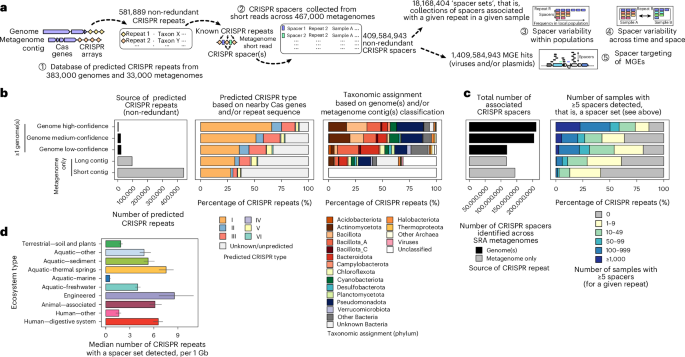
Source data of CRISPR repeat database, repeat identification and dereplication

To build a global database of CRISPR repeat sequences, CRISPR repeats were searched for across 383,318 bacterial and archaeal genomes from NCBI GenBank66 and in contigs from 33,727 public unrestricted metagenome and metatranscriptome assemblies (hereafter, ‘metagenomes’) available in the IMG database67 (accessed February 2023).

For both genomes and metagenomes, Minced v.0.4.2 (https://github.com/ctSkennerton/minced), derived from CRT68, was first run with default parameters to identify potential arrays. For each contig with at least one predicted array, CRISPRCasTyper40 v.1.8.0 was run (option ‘prodigal meta’) to identify which of these repeat regions may represent CRISPR–Cas systems. From the CRISPRCasTyper prediction, a custom Python script (now available as part of ‘SE_run_cctyper.py’ in SpacerExtractor) was applied to refine the predicted repeat sequence from CRISPRCasTyper, specifically looking for cases where the spacers are near-identical at their 5′ and/or 3′ end(s), and extending the repeat as needed. Finally, arrays with the following characteristics were retained: Trusted ‘True’ by CRISPRCasTyper, repeat_identity ≥80, spacer_identity ≤60, spacer_len_sem ≤2, repeat_len ≥23, and repeat_len ≤55. When the repeats were refined by the custom Python scripts, these array features were recalculated except for the ‘Trusted’ value from CRISPRCasTyper. This led to a total of 3,168,155 arrays predicted across genomes and metagenomes.

Repeats were first deduplicated, that is, clustered at 100% nucleotide identity over 100% of both repeats’ lengths (that is, identical lengths), via cd-hit-est69 v.4.8.1 (‘cd-hit-est -d 0 -c 1 -g 0 -aL 1 -aS 1’), which yielded 870,235 unique repeats. Next, these unique repeats were clustered at 100% identity but without a constraint at the repeat length (‘cd-hit-est -d 0 -c 1’). In this second round of clustering, for each genus, only one representative sequence per repeat cluster was kept if this representative sequence represented more than 75% of the repeats in this cluster for this genus. This was done in order to identify and remove potentially mispredicted repeats, that is, repeats identical to other repeats predicted in the same genus but lacking (or having additional) bases at the repeat’s edge. The cut-off of at least 75% of the repeat sequences being strictly identical was used to ensure that a clear consensus sequence was available to be used as a representative. After this second round of clustering, a total of 689,554 unique repeats were obtained.

To further avoid including repeats (and later spacers) that were probably not linked to a CRISPR array, the 689,554 unique repeat sequences were further screened for low complexity based on local composition complexity (LCC) values and k-mer frequency profiles. Specifically, we used the lcc_simp function from the Bio.SeqUtils.lcc Python package and flagged all repeats with LCC < 0.8 as ‘low complexity’. In addition, we used the kcounter package to get counts of k-mers from k = 2 to k = 8, and flagged repeats based on the frequency or counts of the majority k-mer (≥30% at k = 2, ≥20% at k = 3, ≥15% at k = 4, ≥3 occurrences at k = 5 and ≥2 occurrences at k = 6, 7 and 8). This procedure identified 107,628 low-complexity repeats that were filtered out. Finally, all metagenome-derived repeats with a taxonomic assignment to Eukaryota or to viruses outside of the Caudoviricetes order (see below) were considered more likely to originate from a repeat region not associated with a CRISPR array and excluded (n = 315). The final curated database of repeats was composed of 581,889 non-redundant repeats (Supplementary Data File 1 in the Figshare deposit). These repeat sequences were further compared with level 4 CRISPR predictions from CRISPRCasDb70 (14 April 2022 version), and the corresponding CRISPRCasDb identifiers are included in Supplementary Data File 1 in the Figshare deposit when identified.

Taxonomic and CRISPR type assignment process for the CRISPR repeat database

Taxonomic annotation of the repeats (GTDB taxonomy v.r214) was based on genome taxonomy for detections made in a genome or metagenome-assembled genome (MAG), or on contig taxonomy otherwise. For each unique repeat, the taxonomic assignment was based on the lowest common ancestor (LCA) of all identical repeats detected in isolate genomes, if any, or the LCA of MAG contigs larger than 500 kb, if any, or the LCA of all MAG contigs. Because of challenges with binning contigs encoding repeated structures such as CRISPR array loci, we divided genome-based taxonomy into three confidence tiers based on the number and type of detections as follows: (1) the taxonomic assignment of repeats found in four or more genomes of isolates was considered ‘high confidence’ (n = 3,073), (2) the taxonomic assignment of repeats found in four or more MAGs or one or more isolates was considered ‘medium confidence’ (n = 18,572) and (3) the taxonomic assignment of repeats found exclusively in MAGs and in fewer than four genomes was considered ‘low confidence’ (n = 21,838). Repeats exclusively detected in metagenomes (n = 538,406) were classified based on the taxonomic assignment of the corresponding contig in IMG (April 2024), or IMG/VR for contigs predicted to be of viral origin, considering only cases in which this contig classification was based on at least two assigned genes and taking the LCA of all classified contigs for repeats identified across multiple datasets. This yielded an additional 66,327 taxonomic assignments of individual repeats to bacterial (n = 62,076), archaeal (n = 2,987) or phage (Caudoviricetes, n = 1,264) taxa.

In this process, some repeats were assigned to eukaryotic (n = 11) or other viruses (n = 304) and were removed from the final curated database, as mentioned above. The remaining unique repeats (n = 472,079) were not assigned to any taxon. The vast majority of these unclassified repeats (94%, n = 442,389) were exclusively detected on short metagenomic contigs with zero or one predicted genes; that is, the contig consisted almost entirely of the putative CRISPR array without any taxonomically informative region.

Two approaches were used to link the predicted CRISPR repeats to their corresponding CRISPR–Cas system types. CRISPR types were first predicted based on the repeat sequence itself using CRISPRCasTyper40 v.1.8.0 (minimum cut-off of 0.75). In addition, all contigs from which CRISPR repeats were predicted were screened for Cas operons using CRISPRCasTyper40 v.1.8.0. Specifically, individual CRISPR repeats were associated with the type of the closest predicted Cas operon (listed in ‘cas_operons.tab’ by CRISPRCasTyper) if the distance between the CRISPR array and the Cas operon was below 50 kb (Supplementary Data File 3 in the Figshare deposit). Following recent changes to the CRISPR type nomenclature17, Cas operons listed as type II-C2 were assigned as II-D if one of the predicted Cas genes was annotated as Cas4, and II-C otherwise. Each repeat was then assigned to a given CRISPR type either based on a close (<50 kb) Cas operon if available, or based on the sequence-based prediction otherwise. When multiple instances of the same repeat were predicted from different (meta)genomes, the CRISPR type prediction was based on the consensus across a majority (≥50%) of predictions or considered as ‘unknown’ if no type prediction reached this threshold (0.47% of instances).

Selection and metadata collection for public metagenomes

To identify shotgun metagenomic datasets relevant for the CRISPR spacer search, the NCBI SRA database was searched in December 2023 with the following criteria: source field entered as ‘Metagenomic’; the strategy field was not one of ‘Amplicon’, ‘ATAC-seq’, ‘Bisulfite-Seq’, ‘ChIP-Seq’, ‘CLONE’, ‘CLONEEND’, ‘CTS’, ‘Dnase-Hypersensitivity’, ‘EST’, ‘FAIRE-seq’, ‘FINISHING’, ‘FL-cDNA’, ‘GBS’, ‘Hi-C’, ‘miRNA-Seq’, ‘ncRNA-Seq’, ‘POOLCLONE’, ‘RAD-Seq’, ‘RIP-Seq’, ‘RNA-Seq’, ‘Synthetic-Long-Read’, ‘Targeted-Capture’, ‘Tethered Chromatin Conformation Capture’ or ‘Tn-Seq’; the selection field was one of ‘other’, ‘PCR’, ‘RANDOM’, ‘RANDOM PCR’, ‘size fractionation’ or unspecified; and the sequencing platform was one of ‘BGISEQ’ or ‘ILLUMINA’. Datasets indicated as containing fewer than 1,000,000 spots or with an average read length lower than 90 in the SRA metadata were excluded, as were datasets that probably underwent whole-genome amplification, such as those mentioning single-cell sorting or multiple displacement amplification, because whole-genome amplification often leads to inflated predicted spacer diversity, possibly including erroneous spacers due to amplification errors. Read files from all potential datasets to be mined were then downloaded using Kingfisher71, and bbcountunique.sh from BBTools v.39.03 was used to evaluate the uniqueness of the first 25,000 reads. If the percentage of unique reads in this subset was <20%, the dataset was excluded as either an amplicon dataset or a very-low-diversity metagenome. The final list of metagenomes used included 467,018 datasets (Supplementary Data File 2 in the Figshare deposit).

The NCBI Entrez API interface was used to identify the BioSample corresponding to each SRA dataset. Each BioSample was then associated with an ecosystem type using a custom script (‘biosample_to_ecosystem.pl’) based on the information provided in the fields DATA_env_broad_scale, DATA_env_local_scale, DATA_env_medium or DATA_Env_Package, the type of package selected (for example, ‘DATA_human gut environmental package’) or keywords in the fields DATA_sample comment, DATA_host, DATA_isolation_source, DATA_Organism, DATA_Descr or Title. When needed and available, information from the GOLD72 and MGNify73 databases was used to refine the assignment to ecosystem types. This ecosystem information was then aggregated into a simplified classification with 11 ecosystem types: specifically, starting from the detailed classification, ecosystems were ordered based on the number of samples, repeats and spacers observed, and all ecosystems with <1,500 samples or <10 million spacers were grouped with another ecosystem into a broader category (Extended Data Fig. 2). Ultimately, 431,265 datasets (92%) could be associated with one of these 11 simplified ecosystem types, with the majority (59%) of datasets identified as being human-associated.

Comparison of the number and taxonomy of CRISPR repeats across ecosystems

To compare the number of CRISPR repeats detected across samples and ecosystems while accounting for differences in sequencing depth, we randomly subsampled 1,000 metagenomes from each ecosystem, except for Aquatic; Non-marine_Saline_and_Alkaline and Birds-associated for which 500 metagenomes were subsampled, and Fish-associated and Fungi-associated for which 50 metagenomes were subsampled, because of a lower overall number of metagenomes for these ecosystems. For each metagenome, the number of distinct repeats for which a spacer set was detected (see ‘Clustering of spacers and spacer set diversity’) was divided by the total number of bases sequenced in this metagenome. For each ecosystem, the median number of repeats per gigabase (Gb) of metagenome was then calculated. This procedure was repeated 50 times to obtain a distribution of this median number of repeats per Gb across different subsamples for each ecosystem.

The distribution of taxa encoding CRISPR repeats across ecosystems was based on all repeats for which a genus-level taxonomic assignment could be obtained. For each ecosystem, the total number of repeats from each taxon was tallied and converted into a frequency by dividing by the total number of repeats with a genus-level assignment observed in this ecosystem. A heatmap was then prepared using the ggplot274 v.3.5.1 R package and including all genera observed with a frequency ≥2% and/or in the top three highest frequencies for at least one ecosystem. A similar approach was used to calculate the frequency of individual CRISPR types detected across ecosystems.

Initial detection of potential spacers in metagenomic reads

A new approach was designed to identify spacers in metagenomic short-read data, inspired by CRASS35 and CasCollect34. This approach relies on a new component of the BBTools toolkit (‘bbcrisprfinder.sh’), available starting in BBTools v.39.03 (https://sourceforge.net/projects/bbmap/). The entire pipeline is available in a single package named ‘SpacerExtractor’ (https://code.jgi.doe.gov/SRoux/spacerextractor). The version used in this study was SpacerExtractor v.0.8.

The first step in the pipeline identified and extracted potentially relevant reads based on the 581,889 non-redundant CRISPR repeats previously identified (see above) using bbduk.sh (using a FASTA file of these repeats as the ‘ref’ argument, minimum k-mer length of 23, options kfilter, t; maskmiddle, f). Selected reads were then quality-trimmed using bbduk.sh (options ktrim, r; k, 23; mink, 11; hdist, 1; tbo; tpe; minlen, 90; ref, adapters; ftm, 5; maxns, 0; maq, 8) and merged if sequenced as paired-end reads with bbmerge.sh (options mix, nn, t). Next, bbcrisprfinder.sh was used to identify potential ‘repeat–spacer–repeat’ loci in these selected and trimmed reads in two ways: one using the 581,889 non-redundant CRISPR repeats as guides (options k, 13; mm, 1; minrepeats, 2; rmismatches, 1; minspacer, 20; maxspacer, 55; minrepeat, 20; maxrepeat, 55; bruteforce, t; mintailrepeat, 6; rmmt, 0; kref, 13; mmref, 0; maxrefmm, 0) and the other leveraging the de novo detection of ‘repeat–spacer–repeat’ loci from bbcrisprfinder.sh (options k, 13; mm, 1; minrepeats, 2; rmismatches, 1; minspacer, 20; maxspacer, 55; minrepeat, 20; maxrepeat, 55; bruteforce, t, mintailrepeat, 6; rmmt, 0). For the de novo detection, two rounds of detection were performed, with the second using the repeat sequences identified in the first de novo detection as guides. The results of these two different spacer detection steps were then merged to identify the most likely repeat for each read, with priority given to exact complete repeats (two full-length repeats, no mismatches) over exact partial repeats (one full-length repeat and one partial repeat) and over non-exact repeats (some mismatch between the two copies of the repeat). If multiple instances of the same repeat were detected on the same read, the quality of this repeat in this read was taken as the highest quality across all repeats, and the total number of predicted ‘repeat–spacer–repeat’ regions was tallied.

Each read was assigned to a single repeat based on (1) the number of repeat–spacer–repeat regions detected (higher is better), (2) the length of the repeat (higher is better), (3) the quality of the best repeat matches (see above) and (4) the global count of the repeat in the metagenome (higher is better). After linking a read to individual repeats, additional spacers were searched for the same repeat on the read based on the detection of partial repeats on the read’s 5′ and 3′ edges that would have been missed in the first round of detection (minimum 4 bp with no mismatches for considering a partial repeat on a read’s 5′ or 3′ edge). For each metagenome library, this process yielded a list of potential repeats and spacers that were then further refined and quality-checked (Extended Data Fig. 1).

Identification of potentially spurious CRISPR spacers

To remove as many spurious spacer detections as possible, potential spacers were first dereplicated for each metagenome library at 100% nucleotide identity using cd-hit-est69 v.4.8.1 (options -c 1, -G 0, -aL 1, -aS 1). Next, because the repeats and spacers were detected from individual reads and not used in a consensus assembly, a denoising step similar to the one used for 16S rRNA amplicons in DADA275 was performed (Extended Data Fig. 1). Specifically, the repeats detected in a given library were first denoised to identify cases in which a repeat detection probably derived from a sequencing error based on the presence of a near-identical repeat with much higher coverage in the same library. This was done by calculating an expected number of cases in which a given repeat R1 would be observed instead of another repeat R2 due to sequencing error (assuming an error rate of 0.001), considering only cases in which the overall coverage of R2 is higher than that of R1. A P value associated with this expected number of observations under a sequencing error scenario was then calculated based on a Poisson distribution, and a repeat R1 was reclassified as R2 if this P value was ≥0.05, unless the repeat R1 was a singleton (that is, observed in only one read), in which case it was reclassified if the number of expected observations was ≥0.05. When reclassifying repeats, all reads on which the original repeat R1 was predicted were then reprocessed to extract new spacer sequences corresponding to R2.

Next, a similar approach was used to denoise the spacer sequences predicted for each repeat. For each predicted repeat R1, spacers were compared with each other, and a spacer S1 was reclassified as spacer S2 if it was probably derived from S2 given the expected sequencing errors (P ≥ 0.05 or expected number of observations ≥0.05 for singleton spacers). Finally, potentially erroneous spacers were flagged after denoising based on the following criteria (Extended Data Fig. 1): (1) spacer sequences identified as low quality or low complexity, that is, LCC < 0.8 as computed with the Bio.SeqUtils lcc_simp function, the presence of an ambiguous base (‘N’) in the spacer sequence or a high frequency of a given k-mer across the spacer sequence suggestive of a repeat region within the spacer (using the same approach and criteria as for repeats, see above); (2) detection on the edge of a read, that is, spacers for which one repeat is partial and <5 nt; (3) spacers with an outlier length compared with other spacers associated with the same repeat in this sample, that is, with a length either shorter than the first quartile minus 1.5 × IQR or longer than the third quartile plus 1.5 × IQR, based on the length of all spacers for this repeat in this sample; and (4) spacers with unexpectedly conserved 5′ or 3′ ends. Spacer conservation was based on deduplicated spacers and computed as follows: for terminal 2-, 3- and 4-mers, spacer ends were considered as unexpectedly conserved if the most frequent k-mer was found in >50% of deduplicated spacers and with P < 1 × 10−5 when calculating the probability of observing this number of identical k-mers at random under a binomial distribution given the size of the k-mer and the total number of deduplicated k-mers observed. If unexpected spacer end conservation was detected, all spacers associated with this repeat in this sample were ignored. For cases in which identical spacers were associated with multiple repeats in the same metagenome library, the spacer was assigned only to the repeat for which the spacer prediction was the highest quality (that is, no warning flag) or to multiple repeats if the spacer predictions were of identical quality. Finally, spacers flagged as edge, low complexity or low quality, or with an unexpected length or conservation patterns and spacers associated with rare repeats, that is, repeats for which fewer than five spacers in total were detected in the library (ignoring any spacers flagged with one of the previous warnings), were removed from the final set of spacers predicted for each metagenome.

Evaluation of spacer recovery from simulated metagenomes

To evaluate the efficiency and limits of our spacer extraction pipeline, we used a simulation framework similar to Zhang et al.21. First, 200 high-quality genomes (<20 scaffolds) with at least one predicted CRISPR array were randomly selected from the IMG database67. CRISPRCasTyper40 v.1.8.0 with the default parameters was used to establish a ground truth of repeats and spacers for these genomes. Next, art_illumina76 v.2.5.8 was used to simulate reads from these genomes at three different coverage levels (-f parameters set at 0.8×, 10× and 100×) and two different error profiles (-ss, HS25’ and ‘-ss, HS25; -qs, 3; -qs2 3). Other parameters were kept constant (-p; -l, 150; -m, 200; -s, 10). Three different tools were then used on the simulated reads to predict CRISPR spacers: SpacerExtractor v.0.8 (options -m, 0 in ‘filter_hq_spacers’, high-quality spacers only, default parameters otherwise), Crass35 v.1.0.1 (default parameters) and MetaCRAST33 (May 2023 version). For SpacerExtractor, the default repeat database ‘SE_Db_r214GBIMG_0.9’ was used, and for MetaCRAST, the sequence of repeats predicted by CRISPRCasTyper was provided for each genome, while Crass predicts both repeats and spacers de novo. Only repeats present in the SpacerExtractor database were considered in the results; spacers identical (after reverse-complementing if needed) between CRISPRCasTyper and the de novo prediction were considered true positives (TP), spacers predicted for a known repeat but not listed by CRISPRCasTyper were considered false positives (FP) and spacers listed by CRISPRCasTyper but not predicted were considered false negatives (FN). Recall was calculated as TP divided by TP + FN, the false discovery rate as FP divided by FP + TP, and the F1 score as 2 × TP divided by 2 × TP + FP + FN. In addition, another set of metrics was calculated from the de novo spacers predicted by SpacerExtractor after ignoring all singleton spacers (coverage = 1).

Clustering of spacers and spacer set diversity

To build a non-redundant database of spacers, the 794,125,610 curated spacers were clustered at 100% identity using a custom Python script looking for exact string matches (over the entire length) between two spacers or between a spacer and the reverse-complement of another spacer. To evaluate the sequence similarity of singleton spacers to other spacers in the same sample, cd-hit-est v.4.8.1 was used to cluster spacers extracted from each individual sample and each repeat at 95% identity (-c, 0.95) and 80% identity (-c, 0.80).

To define spacer sets, a list of all distinct spacers associated with a given repeat was obtained for each sample and considered the ‘spacer set’ for this repeat in this sample. Each spacer was associated with an estimated depth of coverage on the basis of the number of reads in which this spacer was identified in the corresponding sample. On the basis of the observed distribution of spacer relative coverage within sets, two categories of spacers were empirically defined: ‘common’ spacers as spacers with a number of reads ≥50% of the number of reads of the highest-coverage spacer (that is, the maximum number of reads) in the set, and ‘rare’ spacers as spacers with a number of reads <5% of the number of reads of the spacer with the highest coverage (Extended Data Fig. 4). At the spacer-set level, we categorized spacer sets as low diversity if ≥50% of the spacers in the set were common.

Spacer turnover between samples was evaluated by identifying and tallying the number of identical spacers between spacer sets connected to the same repeat. This was done only for repeats associated with ≥10 sets of ≥10 spacers and at least one spacer with ≥20× coverage (Extended Data Fig. 4). To account for differences in the number of samples in which each repeat was found, the distribution of individual spacers was estimated for a random subset of 10 samples for each set, and the number of samples in which each spacer was observed was tallied. Spacers were considered ‘common’ if they were considered common (coverage ≥50% of the maximum spacer coverage in the corresponding spacer set) in at least one sample.

Samples originating from individual subjects (for host-associated samples) or individual sampling sites (for environmental samples) were identified on the basis of the corresponding BioSample metadata. Specifically, samples with the same value in the ‘DATA_host_subject_id’ field were considered as coming from the same subject, and samples with the same value in the ‘DATA_lat_lon’ field were considered as coming from the same location. Spacer distribution was evaluated using the same approach as previously described: repeats for which spacer sets including ≥10 spacers with at least one spacer with ≥20× coverage were available for ≥10 different sampling dates (to avoid exact replicates) for an individual subject or location were identified. For each of these sets, a random subset of 10 samples from an individual subject or location was selected, and the number of samples in which each spacer was observed was tallied.

Matching spacers to IMG/VR and IMG/PR sequences

Bowtie1 v.1.3.177 was used to identify matches between the 409,584,943 non-redundant spacers and either 5,579,078 IMG/VR v.4.178 high-confidence virus genomes or 699,973 IMG/PR v1 plasmids79. Specifically, a Bowtie1 database was built for IMG/VR v.4.1 and IMG/PR v.1, and spacers were mapped to each database using Bowtie v.1.3.1 with the following options: -a; -v, 3 to report all alignments (‘-a’) for a given spacer and report alignments with up to three mismatches (‘-v 3’) over the whole length of the spacer. The resulting SAM file was then parsed to extract the coordinates of each match along with the number of mismatches (from the ‘NM’ tag), the CIGAR string, and the MD string. Individual alignments of spacers to IMG/VR and IMG/PR sequences were further filtered to remove all alignments overlapping with (1) a low-complexity region in the target, detected with dustmasker v.1.0.0 (package BLAST+ 2.5.0)80 with default parameters or (2) a region predicted as being a CRISPR array, detected with minced v.0.4.2 (default parameters; https://github.com/ctSkennerton/minced) and by mapping sequences from the repeat database built in this study using Bowtie v.1.3.1.

To estimate the number of hits that would be expected from random sequences of a similar length and nucleotide content, we randomly selected a subset of one million spacers with at least one hit in IMG/VR, reversed the sequences, and used the same approach as described above to match to IMG/VR. A total of 309 reversed spacers had a hit against an IMG/VR sequence with zero or one mismatch, suggesting a random hit rate of ~0.03%.

To evaluate the connection between CRISPR targeting and virus–host relationships, we identified 233,982 sequences in IMG/VR with ‘known’ hosts, that is, genomes with a host indicated in the NCBI RefSeq Virus database (n = 3,438) or genomes detected as prophages or proviruses in bacterial or archaeal genomes, respectively (n = 230,544). For these genomes, we specifically compared the host taxonomy as indicated in NCBI RefSeq Virus or in IMG (for prophages/proviruses) with the taxonomy of the repeat for which spacers targeting this genome were identified after converting all taxonomies to GTDB r214. The taxonomies were considered consistent if they were identical from domain to genus rank and inconsistent if different at any rank, for example, pointing to a different genus, family or order.

Prediction of PAMs on the basis of matches to IMG/VR and IMG/PR

For all spacer hits identified with zero or one mismatch across both IMG/VR and IMG/PR, the 10-bp regions upstream and downstream of the match were extracted. For each repeat cluster, surrounding regions across all spacer hits were deduplicated such that only one copy of each region was retained when both upstream and downstream 10-bp sequences were identical. Then, conserved nucleotides observed in ≥75% of the distinct set of regions for a given repeat cluster were identified. These conserved positions were then compared with a set of known PAMs previously described in the literature46,47. Only cases with at least two conserved positions were considered, except for repeats predicted as being type II for which one-position motifs were considered on the basis of known PAMs. Because the orientation of the repeat is ambiguous in our analysis, all PAMs were assumed to be upstream of the spacer, except for type II repeats, where PAMs were assumed to be downstream of the spacer. If a conserved region was observed on the opposite strand, for example, upstream of a type II repeat or downstream of a non-type II repeat, the sequence was reverse-complemented for the purpose of PAM detection. Finally, the known PAMs were completed by motifs observed in ≥5% of neighbourhoods, which were typically minor variants of known PAM motifs (Extended Data Fig. 7).

Additional annotation, feature prediction and comparison of IMG/VR genomes

Information on virus genomes, including original ecosystem and taxonomic assignment, was obtained from the IMG/VR v.4 database78. In addition, a lifestyle prediction was performed, as well as the identification of putative DGRs and anti-CRISPR genes. For lifestyle prediction, we identified all sequences for which the IMG annotation included a gene with a product mentioning ‘integrase’ or ‘recombinase’, and conducted additional searches against a published database of integrase Hidden Markov Model (HMM) profiles81, as well as all HMM profiles annotated as integrase in the PHROG82 v.4 database (hmmsearch83 v.3.3.2, score ≥ 50 and expected value (E-value) of ≤1.0 × 10−5; default parameters otherwise). All sequences predicted to encode an integrase/recombinase on the basis of one or more of these annotations were predicted as having a ‘temperate’ lifestyle. For DGRs, the approach used in https://bitbucket.org/srouxjgi/dgr_scripts/src/master/DGR_identification/ (ref. 84) was used, with the detection of a putative DGR reverse transcriptase on the basis of a collection of HMM profiles (hmmsearch83 v.3.3.2, score ≥ 50 and E ≤ 1.0 × 10−5; default parameters otherwise) followed by a custom script to detect likely DGRs on the basis of the presence of a nearby template repeat and variable repeat, respectively, structure. Finally, anti-CRISPR genes were searched on the basis of the APIS database85 (June 2024) using diamond86 v.2.1.8 (parameters --max-target-seqs, 999999999; score, ≥50; E ≤ 1.0 × 10−5; minimum coverage of 80% for query and target; default parameters otherwise) and hmmsearch83 v.3.3.2 (minimum score of 50 and maximum E = 1.0× 10−5; default parameters otherwise).

To compare the functional annotation of targeted and untargeted regions in viruses, subsamples of 1,000,000 spacers matching a single vOTU and 1,000,000 spacers matching multiple vOTUs were selected. For the corresponding targets, the predicted CDSs overlapping the spacer hits were extracted from the IMG annotation, and annotated with the PHROG82 v.4 database using MMseqs287 v.14.7e284 (easy-search function, score ≥ 50, E ≤ 1.0 × 10−5, default parameters otherwise). Genes were considered functionally annotated if they showed one or more hits against the PHROG database.

To evaluate the similarity between sequences targeted by the same spacer, a set of 2,000,000 spacers matching multiple high-quality virus genomes was randomly selected, and genomes targeted by each spacer were compared all-versus-all using lz-ani88 v.1.0.1 (all2all function, default parameters). For each spacer, the largest distance (that is, 1 − global average nucleotide identity) between a pair of high-quality virus genomes was taken as the maximum distance between targets for this spacer.

Definition of targeting patterns and identification of associated viral features

For IMG/VR matches, patterns of spacer targeting (that is, the number of spacers matching a target, the percentage of target covered, the number of spacer hits for different numbers of mismatches between spacer and target and the targeting by prokaryotic host taxon) were calculated for prokaryotic viruses only. Specifically, only genomes assigned to Tokiviricetes, Caudoviricetes, Faserviricetes, Malgrandaviricetes, Huolimaviricetes, Leviviricetes, Tectiliviricetes or Laserviricetes classes were considered for these analyses, except sequences assigned to the Rowavirales order (that is, adenoviruses), which were specifically excluded as this taxon contains eukaryotic viruses within the Tectiliviricetes class of bacteriophages and archeoviruses.

To evaluate the level of targeting of individual viruses by individual CRISPR repeats, we analysed the collection of spacer hits on the basis of all spacers collected across all samples for a given repeat to a given virus genome. The total virus genome coverage by spacers was calculated as the number of positions to which at least one spacer from this repeat had a hit with zero or one mismatch, divided by the total length of the virus genome.

For virus–repeat pairs including ≥10 spacer hits with zero or one mismatch covering ≥200 bp and for which the virus genome is of ‘high quality’ (that is, ≥90% completeness), the spacer hits with two or three mismatches were extracted from the same Bowtie1 mapping (see above) and tallied to be compared with the number of spacers matching the same virus genome with zero or one mismatch. To summarize these mismatch profiles, we computed the ratio between the number of spacer hits with zero or one mismatch divided by the total number of spacer hits (zero, one, two or three mismatches). This ratio was then used to empirically define three categories of virus–repeat pairs: ‘mostly distant’ if the ratio was <0.5, that is, a majority of spacer hits are found with two or three mismatches, ‘mostly near-exact’ if the ratio was ≥0.8, that is, more than 80% of the spacer hits show zero or one mismatch, or ‘mixed’ for ratios between 0.5 and 0.8 (Fig. 4d).

Analysis of targeting patterns for viruses with a potentially broad host range

When exploring the taxonomic range of CRISPR repeats targeting individual viruses, only repeats with a taxonomic assignment of medium or high confidence were used (see ‘Taxonomic and CRISPR type assignment process for the CRISPR repeat database’). Next, virus sequences from two previous studies37,39 that highlighted potential broad-range targeting were re-analysed using this set of taxonomically assigned spacers. The sequences of 547 and 13,404 viruses, respectively, were collected, and spacer mapping using the same Bowtie1-based approach was performed for the same non-redundant set of spacers (see above). Spacer hits were collated using the same approach as previously described to calculate the overall coverage and mismatch profile for each virus–taxon pair.

For virus–taxon network representation, two selection criteria were applied. First, the specific virus sequences that had been previously highlighted as targeted by multiple phyla37,39 were selected and included in the virus–taxon network if also connected to multiple phyla on the basis of hits from the global spacer database (Fig. 5a). Next, virus sequences from the George et al. dataset37 not already included in Fig. 5a but connected to repeats from different phyla with 10 or more hits on the basis of the new global spacer database were included in a separate network (Fig. 5b). In both cases, Cytoscape89 v.3.10.1 was used to display the networks.

Visualization and statistical tests

All visualization and statistical tests were performed using R v.4.3.3 (29 February 2024), except for the networks, which were displayed with Cytoscape v.3.10.1.

Reporting summary

Further information on research design is available in the Nature Portfolio Reporting Summary linked to this article.