Sentinel data were assigned a location on the basis of the closest recorded fix in time within a cut-off of 2 min—any sentinel data without a corresponding location within 2 min were not analysed.
Over the study period, we observed 728 unique sleeping locations being used by mongoose groups (Supplementary Fig.
Models investigating the effect of relative neighbour group size (Supplementary Tables 2–5) were fitted with fixed factors for both a linear and quadratic effect of relative neighbour group size.
Both were modelled identically, with fixed factors included for normalized difference vegetation index, population density, time of year, mean group size (mean of the two neighbours in the pair) and the relative group size of the two neighbours.
2b), we adjusted these plotted values by the estimated group-size effect, given the inherent relationship between absolute and relative group size (see Supplementary Fig.
Study species
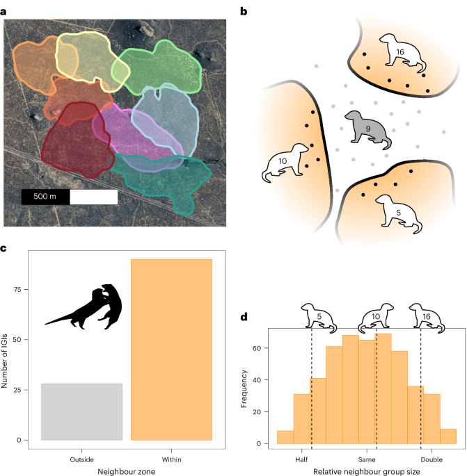
Dwarf mongooses are sexually monomorphic, group-living, territorial mammals found throughout Southern Africa32,50. They live in cooperatively breeding groups comprising a dominant breeding pair, their offspring and immigrants, with an overall balanced sex ratio32. Both sexes disperse and immigrate into new groups resulting in a relatively even relatedness structure between sexes32. Members of a group move cohesively in the environment; larger groups travel further daily distances and cover more area, ultimately resulting in larger groups occupying larger areas38. Groups routinely deposit scent marks at regularly used latrine sites, which fall predominantly near home range boundaries36,43. While groups do not patrol boundaries in the same way as some other species56,57, they regularly show directed movement to these marking locations, and the same latrine sites have been used by pairs of neighbouring groups over multiple years (DMRP, unpublished data). Groups engage directly with neighbours when they are encountered; these events are termed IGIs33,36,38. When IGIs occur, both male and female adults participate at equivalent rates, and the majority of IGIs result in agonistic physical interactions between the groups, occasionally resulting in injury and even mortality34; unlike some species, IGIs very rarely involve affiliative behaviour between members of different groups, and there is no evidence for extra-group paternity as seen in closely related species6,58. Groups may use indirect cues (for example, scent marks) and memories of past interactions to assess neighbour group size and the likelihood of encounter, even when there are no direct indicators that another group is currently nearby43,59.
In addition to the threat posed by neighbouring conspecific groups, dwarf mongooses are also depredated by a variety of diurnal and crepuscular predators, including many mammals and birds of prey35. As an adaptation to such a predator-rich landscape, dwarf mongooses perform coordinated vigilance known as sentinel behaviour, where one individual climbs to an elevated position and watches for danger35,60. During their bout, sentinels often announce their presence to the group by producing vocalizations termed surveillance calls, enabling foragers to reduce their vigilance37,39. Sentinel behaviour increases in response to the simulation of intergroup intrusions36,49, suggesting that sentinels can also act to detect potentially threatening conspecifics as well as heterospecifics. Dwarf mongooses are strictly diurnal and rely on burrows, mostly excavated termite mounds, in which to spend the night and avoid crepuscular and nocturnal predators38,61. Groups routinely switch burrows38, and burrows are found evenly distributed throughout the habitat (Supplementary Fig. 2).
Ethics
Work was conducted under permission from the Limpopo Department of Economic Development, Environment and Tourism (permit no. 001CPM403-00013). Ethical approval was granted from the University of Pretoria, South Africa (Animal Ethics Committee: NAS321/2022) and the University of Bristol, UK (Animal Welfare and Ethics Review Body: UB/11/038), and the study was performed in line with The Association for the Study of Animal Behaviour guidelines for the ethical treatment of animals62.
Data collection
All data were collected at Sorabi Rock Lodge, Limpopo Province, South Africa (24.211° S, 30.775° E), as part of the long-term Dwarf Mongoose Research Project. Data were collected between September 2013 and September 2023 from 12 groups of wild, habituated dwarf mongooses. During the winter months (~May–September), groups were followed for the entire day, from when they first emerged in the morning from the overnight sleeping burrow until they returned and went into a sleeping burrow in the evening. During the hot summer months (~October–April), groups were followed for ~3 h from when they left the overnight sleeping burrow, at which point the observer would leave the group during the heat of the day, returning to follow the group for 2–3 h before they returned to a sleeping burrow in the evening. This summer pattern of data collection was facilitated by mongooses becoming inactive in the heat of the day, often retreating below ground at a day refuge until later in the afternoon when it became cooler. Groups were observed for a mean of 9.2 days per month over the study period, usually in 2–3-day blocks38.
Observers collected three core datasets, which we use in this study: life-history, movement and behaviour data. The identity of all present group members was recorded during every observation session, enabled by the periodic application of unique blonde hair-dye marks for individual recognition. Birth data were collected to enable accurate designation of adult group members (individuals >1 year old) and therefore calculate adult group sizes. To generate a group size for neighbours on days when we did not visit a group, we used linear interpolation from the observed group sizes on either side of the unknown date. Observers continually recorded location data by positioning themselves close to the centroid of the group, taking the group track on a Garmin Etrex 10 (Garmin) handheld GPS device recording fixes typically at <3 m of accuracy38. We use these data to generate UDs and movement metrics, and to infer the locations of spatially anchored behavioural observations (that is, sentinel bouts and burrow uses).
Multiple behaviours were recorded during observation sessions. All observed IGIs were noted, and their location was logged with GPS. Sentinel behaviour was recorded through a combination of routine scan samples and ad libitum observations35,40. Scan samples were conducted every 30 min to assess whether a sentinel was present. At all times, other sentinel bouts were recorded with more detailed information on the duration of the bout and whether the sentinel announced its presence through vocalizations37; for both duration and vocalization data, only sentinel bouts where the observer witnessed the full bout were used for analysis. The location of sentinel scan samples and ad libitum bouts was inferred from daily GPS tracks. Sentinel data were assigned a location on the basis of the closest recorded fix in time within a cut-off of 2 min—any sentinel data without a corresponding location within 2 min were not analysed. Return time to the evening sleeping burrow was recorded as the time that 50% of the adult group members returned to the burrow that they subsequently went to sleep in. The location of all known burrows where timing data were obtained was logged with GPS. Over the study period, we observed 728 unique sleeping locations being used by mongoose groups (Supplementary Fig. 2).
Data processing and analysis
All processing and analyses were conducted in R63 (version 4.5.1). First, we subsampled all GPS data to a target rate of one fix per minute to generate a standardized sampling rate, using the method outlined in ref. 64. Throughout, we calculated UDs using the most recent 90 days of GPS data for those groups with a minimum of 20 days of data available (as in ref. 38), using functions from the R package ‘adehabitatHR’ 65 (version 0.4.22). A period of 90 days was chosen as a compromise between capturing enough data to generate meaningful UDs while keeping assessed areas recent enough for the specific aims of the study. When generating UDs, we chose to use ‘standard’ (not autocorrelation corrected) kernel density estimation (KDE) to ensure our estimates of where mongoose groups had moved in the previous 90 days was conservative. When analysing movement data from our study system, we have previously found that estimating space use using autocorrelation-corrected KDE methods has resulted in estimation of home range areas ~1.4× larger than those estimated using KDE methods, including areas we have never seen groups over many years of observation38. This reduced the estimated used space (and therefore number of included behavioural data points carried into analysis) relative to calculating overlaps using an autocorrelation-corrected KDE method (implemented through continuous time movement models66). However, it ensured higher confidence in our assessment that a certain location was observed to be within the space recently used by a neighbour.
To assess the effects of relative neighbour group size on behaviour, we took each day with a recorded behavioural observation (movement tracking, sentinel observation and/or burrow use in the evening) and isolated those for each focal group that fell within the 95% UD of a neighbour (Fig. 1b), termed the neighbour zone, using functions from the R package ‘sf’67 (version 1.0–24). For these behavioural data in neighbour zones, we calculated the relative neighbour group size for each identified neighbour as the base 10 logarithm of neighbour group size/focal group size, such that relative group-size differences were centred on, and symmetrical around, 0 (for example, |log 10 (2)| = |log 10 (1/2)|; Fig. 1d). Models investigating the effect of relative neighbour group size (Supplementary Tables 2–5) were fitted with fixed factors for both a linear and quadratic effect of relative neighbour group size. These models controlled for focal group size as a fixed factor, as well as being fit with random intercepts for focal group and neighbour group identity and random slopes for the effects of focal group size and relative neighbour group size within focal group identity. Random terms showing zero variance were kept in models, and the s.d. for these terms is noted as 0.000 in Supplementary Tables. To assess the effects of location within the home range on behaviour, we assigned all recorded behavioural observations a location within the focal group’s home range using the same GPS method as above. All observations within the 50% UD were assigned as occurring in the ‘core’ area, and all observations outside the 75% UD were assigned as occurring in the ‘edge’ area (Fig. 3a). Observations that fell in the buffer zone between core and edge (that is, 50–75% UD) were not analysed. Models investigating changes in behaviour relative to location within the home range (Supplementary Tables 6–8), not just restricted to neighbour zones, were fitted with fixed terms for absolute group size and location within the home range, a random intercept for group identity as well as random slopes for group size and location within-group identity. While groups consistently had unhabituated neighbours (for example, outer edges in Fig. 1a), our approaches are not impacted by these groups: for relative group-size analyses, we used only data from zones with known neighbours; the location-based analyses are egocentric and are therefore agnostic to whether a potential neighbour is in the habituated study population or not.
Before statistical modelling, we removed outliers (data points more than three s.d. from the mean) to enhance model fit and prevent models from violating assumptions. We scaled all absolute group-size, bout duration and overlap-size predictors to a mean of 0 and an s.d. of 1 to aid model fitting. We assessed significance of terms using likelihood ratio tests between the final model with and without the term of interest. Nonsignificant quadratic terms were removed to allow interpretation of the linear term—the model with significant quadratic term/without nonsignificant quadratic term was considered the final model, with all other a priori modelled predictors retained. Effect sizes are taken from the model summaries and transformed to the original data scale where appropriate.
All presented models were run using functions from the ‘lme4’68 (version 1.1–38) and ‘glmmTMB’69 (version 1.1.14) packages. We checked all model assumptions using diagnostic tools from the ‘DHARMa’ package70 (version 0.0.7), with variance inflation below 3 for all terms in all models, as checked using the vif() function from the ‘car’ package (version 3.1–5). We checked model residuals for temporal autocorrelation to ensure behaviour was not significantly correlated across days. In addition, we found little evidence that response metrics were correlated within group and day (Supplementary Fig. 3). The likelihood that a sentinel vocalized is weakly but significantly correlated with both the likelihood of a sentinel being present (r = 0.22, P < 0.001) and the duration of sentinel bouts (r = 0.17, P < 0.001). Models for vocalization include the log of bout duration as a covariate, as these variables are both gathered at the single bout level, determined by the log-linear relationship between bout durations and vocalization likelihood (Supplementary Fig. 4), whereas likelihood of a sentinel being present is from the independent scan-sample dataset. By nature, movement speed and area covered are also significantly correlated (r = 0.25, P < 0.001) but have the potential to highlight nuanced differences in movement behaviour and are therefore interpreted together38.
To assess the factors that influenced the extent to which groups overlap in their space use, we calculated 95% UDs for 3-month blocks (January–March, April–June, July–September and October–December) for all groups. We then calculated the size of areas that overlapped between neighbouring pairs, proportional to the full 95% UD of both groups. To control for potential impacts of environmental productivity on overlap size38, we took the 3-month mean normalized difference vegetation index value for the study area, taken from the MODIS product MOD13Q171: 16-day, 250 m × 250 m resolution (as in ref. 38), using functions from the ‘MODISTools’ R package72 (version 1.1.6). Similarly, to control for population density, which could influence space use and overlap size73, we summed the size of all measured group 95% UDs and divided by the number of individuals over 1 year old to achieve a metric of adult mongooses per ha. For this analysis, absolute group size was calculated as the mean linear interpolation of the number of adult individuals across the 3-month block (mean of 7.9, s.d. of 2.0, range of 4.4–13.4, N = 274 group blocks). As each overlap can generate two proportional areas (overlap/group 1 versus overlap/group 2), we ran two near-identical models, from the perspective of the larger and smaller groups in each pair, respectively, to avoid pseudo-replication inflating our sample size. Both were modelled identically, with fixed factors included for normalized difference vegetation index, population density, time of year, mean group size (mean of the two neighbours in the pair) and the relative group size of the two neighbours. Both models yielded qualitatively identical results (Supplementary Table 1); we present those from the perspective of the larger group in the main text.
When assessing the likelihood of entering, and proportion of time spent within, neighbour zones, data were summarized at the level of the month. For each group, we took the proportion of days in which any fix was located within a neighbour zone with each neighbour, with a minimum of 5 days observed in a given month. We also analysed the proportion of all fixes observed in the neighbour zone with each specific neighbour, again with a minimum of five observation days per month. These were analysed using generalized linear mixed models (GLMMs) with gamma error and a log link function (Supplementary Table 2). All models contained an additional fixed factor for the proportional size of the overlap between the home ranges of the focal group with a given neighbour, relative to the home range size of the focal, to control for the effect of differences in mutual space use between groups.
We calculated movement speed for each fix (as distance/time since last fix) that was >50 and <70 s since its predecessor. The mean of each speed was then taken to generate the movement-speed metric. We determined unique area covered per unit time as the number of unique 20-m width hexagonal cells the track intersected divided by the time taken (the full method can be found in ref. 38. Both movement speed and unique area covered per unit time were modelled as linear mixed models (LMMs) with log-transformed response data (Supplementary Tables 3 and 6). Models investigating home range location contained observation day as an additional random intercept to capture the non-independence of track segments from within the same day (Supplementary Table 6); for this analysis, we only included days that had track segments in both core and edge areas.
Models investigating sentinel presence in a scan sample and whether a sentinel vocalized during a given bout (each with responses of yes or no; Supplementary Tables 4a,c and 7a,c) were analysed as GLMMs with a binomial error structure and logit link function. Models investigating the duration of sentinel bouts (Supplementary Tables 4b and 7b) were run as LMMs with the log-transformed bout duration fitted as the response term. Models investigating vocalization had bout duration (logged) fitted as an additional fixed term. All sentinel models contained an additional random intercept for the specific observation session to account for the non-independence of multiple data points taken in a single session.
We took all days in which a group was recorded entering a neighbour zone and noted whether they slept at a burrow in the neighbour zone that evening. This was modelled as a binomial GLMM with a logit link function (Supplementary Table 5a), with an additional fixed factor for the proportional size of the overlap between the focal group and given neighbour. Models investigating return time to the evening sleeping burrow (Supplementary Tables 5b and 8) were run as LMMs with log-transformed response data with a small constant added to all values before transformation to prevent negative values, thus enabling the transformation.
To help visualize our main effects, we added discretized raw data to our plots of model-estimated effects and CIs (Fig. 2). For models investigating relative group-size effects, where there is also a main effect of group size with P < 0.1 (Fig. 2b), we adjusted these plotted values by the estimated group-size effect, given the inherent relationship between absolute and relative group size (see Supplementary Fig. 1 for further details). Model output tables in Supplementary Information represent those values generated directly from running R code, whereas effect sizes and figures represent the back-transformation of these values, including accounting for any link functions in models and scaling of variables.
Reporting summary
Further information on research design is available in the Nature Portfolio Reporting Summary linked to this article.