A vector-based strategy for olfactory navigation in Drosophila

Fly husbandry

Flies were maintained at 23–25 °C and 60–70% relative humidity under a 12-h light–dark cycle. The quality and composition of the fly food was a key factor for eliciting robust edge-tracking behaviour in tethered flies, particularly during imaging experiments. We found that flies that were raised for several generations on Wurzburg food39 exhibited robust edge tracking more consistently than did those raised on standard cornmeal–agar–molasses food. All behavioural experiments were performed using starved flies, which were removed from food and placed in vials containing only a water-soaked KimWipe or cotton plug for 16–24 h before tethering. For optogenetic experiments, flies were reared in complete darkness. Two days before an experiment, one-to-two-day old flies were transferred to a food vial containing 0.4 mM all-trans-retinal (Sigma, R2500). Sixteen to twenty-four hours before an experiment, flies were removed from food and placed in a vial containing a Kimwipe soaked in 1–2 ml of 0.2 mM all-trans-retinal in water.

Detailed fly genotypes

For all behavioural experiments examining edge tracking of an odour plume (Figs. 1, 2, 4 and 5 and Extended Data Figs. 1–3, 5–7, 9, 11 and 12), we used Canton-S. For perturbations of EPG neurons (Fig. 3), we used the SS00098 EPG split Gal4 line: 19G02-p65AD/+; R22E04-DBD/UAS-GtACR1-EYFP. For functional imaging of EPG neurons (Figs. 3 and 6 and Extended Data Fig. 14), we used the 60D05-Gal4 driver: UAS-jGCaMP7f/+; 60D05-Gal4/+. For perturbations of FC2 neurons (Fig. 6 and Extended Data Fig. 14), we used VT065306-AD; VT029306-DBD/UAS-GtACR1-EYFP. For functional recording of FC2 neurons (Fig. 6 and Extended Data Fig. 14) we used VT065306-AD/UAS-syt-jGCaMP7f; VT029306-DBD/60D05-Gal4. For optogenetic activation of olfactory sensory neurons (Extended Data Fig. 4), we used: UAS-Chrimson.mVenus/Orco-GAL4, w1118 UAS-CsChrimson.mVenus, Orco-GAL4, w*.

Drosophila stock sources. EPG split line: 19G02-p65ADZp (in attP40); R22E04-ZpGdbd (in attP2) (Bloomington Drosophila Stock Center (BDSC) 93169); FC2 split line: VT065306-AD; VT029306-DBD (gift from G. Maimon); R60D05-Gal4 (BDSC 39247); 10XUAS-sytGCaMP7f (attP2) (BDSC 94619); 20XUAS-IVS-CsChrimson.mVenus(attP18) (BDSC 55134); Orco-GAL4.C(142t52.1), w[*] (BDSC 23909); UAS-GtACR1.d.EYFP(attP2) (BDSC 92983); 20XUAS-IVS-jGCaMP7s(VK00005) (BDSC 79032).

Fly tethering and dissection

All assays were performed using 1–5-day old female flies. Flies were briefly anaesthetized (less than 10 s) using CO 2 and tethered to a custom-milled fly-plate similar to what has been previously described56. Flies were mounted to the fly-plate using a strand of hair or a single paintbrush bristle, which was used to secure their heads and subsequently their bodies to the plate before gluing the eyes and thorax using UV-curable glue. In all assays, the filament was removed after successful tethering and flies were placed in a dark, climate-controlled space (25 °C, 40–60% relative humidity) to recover for 15–30 min before the start of the experiment. Flies were then transferred to the closed-loop apparatus and allowed to walk freely on the ball for at least 15 min before experiments.

For functional imaging experiments, fly preparation varied accordingly. After tethering, the proximal portion of the extended proboscis was glued to minimize movement during recording while allowing the distal portion of the mouthparts to move freely during experiments. Flies were provided a recovery period of 30–120 min after tethering. After the recovery period, the fly-plate was then filled with saline (108 mM NaCl, 5 mM KCl, 2 mM CaCl 2 , 8.2 mM MgCl 2 , 4 mM NaHCO 3 , 1 mM NaH 2 PO 4 , 5 mM trehalose, 10 mM sucrose and 5 mM HEPES sodium salt, pH 7.5 with osmolarity adjusted to 275 mOsm). The cuticle covering the posterior portion of the brain was then cut using a 30-gauge needle and removed using forceps to facilitate optical access to central complex structures. Obstructing trachea were removed taking care to not damage the antennae or the antennal nerves. Flies were subsequently transferred and allowed to walk on the ball for at least 15 min.

Preparation of the olfactory environment

A virtual olfactory environment was created for walking tethered flies using a previously described16 closed-loop olfactory system with the addition of custom Python scripts that allowed for two-dimensional (2D) rendering of odour plumes.

Tethered locomotion

For tethered locomotion experiments, a spherical treadmill based on previous studies was designed. A 6.0–6.5-mm-diameter ball was shaped from LAST-A-FOAM FR-4618 (General Plastics) by a custom-made steel concave file. The ball rested in an aluminium base with a concave hemisphere 6.75 mm in diameter with a 1-mm channel drilled through the bottom and connected to an airflow. The ball was recorded at 60–61 frames per second using a Point Grey Firefly camera (Firefly MV 0.3 MP Mono USB 2.0, Point Grey, FMVU03MTM-CS) with an Infinity lens (94-mm focal length) focused on the ball, with illumination from infrared LED lights. Ball rotation was calculated in real time using FicTrac software57 running on computers with processor speeds of at least 3 GHz.

Closed-loop arena

The heading of the fly, as calculated by FicTrac, was transmitted to a RaspberryPi 4 through a serial port. Custom Python code was used to translate heading into tube position, controlled by motors, as described below. The closed-loop air delivery system was custom designed using OnShape (https://www.onshape.com) and 3D printed using VisiJet Crystal material at XHD resolution in a 3D Systems ProJet 3510 HD Plus. O-ring outside dimension and inside dimension gland surfaces were designed with excess material for printing and then manually modified on a lathe for improved RMS (surface) finishing. The 360° tube rotation was driven by a bipolar stepper motor (SureStep DC integrated NEMA 17 stepper) controlled through an integrated driver and coupled by a Dust-Free Timing Belt (XL Series, 1/4″ width, McMaster-Carr, 1679K121, trade no. 130 × L025) to the rotating tube system, which rotated mounted on an Ultra-Corrosion-Resistant Stainless Steel Ball Bearing (3/4″ shaft diameter, 1-5/8″ inner diameter, McMaster-Carr, 5908K19). The air channel was kept airtight using oil-resistant O-rings (1/16″ fractional width, dash no. 020, McMaster-Carr, 2418T126). Motor rotation was measured by a rotary encoder (CUI Devices, AMT10 Series) that was used to correct for skipped steps.

Airflow and odour delivery

Odour delivery was achieved by directing a continuous stream of humidified clean air through a 2-mm-diameter tube made of VisiJet Crystal material directed at the fly’s antennae. An anemometer (Kanomax 6006-DE) was used to ensure that airspeeds reaching the fly were maintained at 15–25 cm s−1. Air to the system was first passed through a charcoal filter and humidified by bubbling the air through a deionized water reservoir. The airflow was then split between the spherical treadmill and three mass flow controllers (MFCs; Alicat, MC-Series, 1000SCCM). Downstream of each MFC, air passed through the headspace of odour vials containing either ACV (Heinz) or deionized water. The ratio of air entering each vial was dependent on the fly’s position relative to the odour plume, such that when a fly is outside the boundaries of the plume, 100% of the air is directed into the water vial; when the fly is within the boundaries of the plume, the air is directed at an experimenter-determined ratio between the water vial and the odour vials. Air streams coming from the odour vials then merge with a Y-connector before entering the air delivery system. Thus, by controlling how much of the air passes through each vial, the MFCs control the total odour concentration of the airstream reaching the fly. The MFCs were controlled using a RaspberryPi 4 running custom Python scripts.

Optogenetic stimulation

All optogenetic experiments were done on flies with intact cuticles. Flies were reared in the dark, transferred to retinal food and tethered as described above. For optogenetic experiments, a fibre-coupled LED was controlled by a T-cube LED driver (Thorlabs, LEDD1B) to deliver light to the fly’s head in closed loop with its behaviour. For the activation of Orco+ sensory neurons, a 660-nm (red) LED (Thorlabs M660FP1) was turned on (0.863 μW mm−2) when the fly was inside the fictive odour plume. For EPG inhibition experiments, a 530-nm (green) LED (Thorlabs M530F2) was turned on (0.752 μW mm−2) for the duration of the entire trial.

Closed-loop parameters

Behavioural measurements (sampled at 60 Hz) were determined by the rotation of the foam ball and obtained from FicTrac (x position, y position, heading, roll, pitch and yaw). These were saved alongside MFC flow values, experimental variables (odour on, LED on) and a time stamp in a single .log file.

Edge-tracking behavioural assays

Tethered behavioural assays were performed in a dark, climate-controlled room (25–27 °C, 40–60% relative humidity). The closed-loop olfactory system was enclosed in a black tarpaulin as a further shield from other potential light sources, such as computer monitors and indicator lights on system hardware. To prevent odour build-up in the enclosed space, a vacuum line (60 cm s−1) was placed at the back of the enclosure as an exhaust. Unless otherwise stated, all experiments started with a 2–5-min baseline period in which flies walked in clean air delivered in closed loop. At the end of this baseline period, flies were placed at the centre of the odour plume’s short axis, with the exception of the 90° plume, in which flies were placed at the centre of the odour plume’s long axis. The geometry of the plume (0°, 45° or 90°) was determined before the start of the experiment. Unless otherwise stated, each plume’s short axis measured 50 mm and each long axis 1,000 mm. For EPG and FC2 imaging experiments, the plume’s short axis was 10 mm. For EPG and FC2 silencing experiments, all flies completed paired LED-on and LED-off trials in pseudo-random order. For the jumping-plume experiments in Figs. 2d,h, 3e,f and 6 and Extended Data Figs. 5i, 6, 7 and 14, the edge of the plume was shifted 20 mm in the direction opposite to the fly’s heading as the fly exited the plume. Owing to the propensity of flies to engage in straighter trajectories because of the heat of the two-photon laser6, during functional imaging of FC2 neurons (Fig. 6 and Extended Data Fig. 14), once the fly had made 20 plume entries, the plume was jumped 3 mm on every third subsequent entry. For all experiments, trials were terminated if one of these three criteria was met: (1) the fly travelled the length of the long axis of the plume provided (1,000 mm), except in the case of FC2 imaging, in which experiments were terminated at 2,000 s; (2) the fly travelled more than 500 mm perpendicular to the plume’s edge; (3) the fly travelled 100 mm downwind from its starting position on the plume.

A small fraction of tethered flies (less than 10%) were excluded from the study because they did not acclimate to walking on the ball, because they did not show a behavioural response to ACV (by turning upwind and increasing their speed) or because continuous tracking of the trajectory was lost by FicTrac.

Odour concentration-gradient plumes

Gradient plumes were created with the same dimensions (50 mm by 1,000 mm) but featured one of three odour concentration gradients. (1) Vertical plume with increasing upwind odour concentration: odour concentration increased linearly in the upwind direction, starting at 10% ACV at the plume’s downwind end (0 mm) and reaching 100% ACV at the upwind end (1,000 mm). (2) Vertical plume with decreasing upwind odour concentration: odour concentration decreased linearly in the upwind direction, starting at 100% ACV at the downwind end (0 mm) and diminishing to 10% ACV at the upwind end (1,000 mm). (3) 90° plume with crosswind odour concentration gradient: odour concentration varied linearly along the lateral axis, increasing from 10% to 100% ACV in one crosswind direction or decreasing from 100% to 10% ACV in the opposite direction over 1,000 mm. Flies were at first positioned at the interface between these two gradients, allowing them to track up or down the concentration gradient in the crosswind direction.

Graded lateral plumes

Plumes with graded lateral concentration profiles followed a Gaussian profile characteristic of naturalistic plume envelopes. To make these plumes most comparable to the 50-mm constant-concentration odour corridor, the peak odour concentration was set to 20% at the plume’s midline, and the plume’s width was adjusted to 160 mm so that the half-maximal concentration occurred at ±25 mm from the plume’s midline. Flies tested in a plume with a graded lateral boundary were also tested in a plume with a sharp lateral boundary (Extended Data Fig. 3) in pseudo-random order.

Optogenetically generated fictive odour plumes

Fictive odour plumes were the same dimensions as a vertical odour plume (50 mm by 1,000 mm). Flies were positioned in the centre of the plume’s short axis and optogenetic stimulation was provided by a 660-nm LED whenever the fly was within the plume’s boundaries.

Disappearing plumes

Flies tracked a constant-concentration plume for 10 min. After this period, during their first trajectory outside the plume, the plume was removed, leaving the fly walking in closed-loop wind without further olfactory input.

Dynamic plumes

Flies were presented with a looped video of a previously recorded surface plume that was binarized to match the composition of concentrations in odour corridors. The video spatial dimensions were scaled up by bicubic interpolation to provide a larger stimulus in which flies were likely to make more than one to five returns (total alongwind length was 2,030 mm instead of the original 300 mm), and the replay speed was scaled down (see ‘Dynamic plume analysis’). Flies were initialized at a position 1,700 mm downwind and at the centre line of the fictive source. During exploration, odour delivery was referenced to the fly’s spatial position relative to the video X, Y dimensions and to the presence of odour at that referenced pixel in the frame of the T dimension of the video matching the experimental time elapsed. Given the irregular plume structure and the time-varying intermittency of odour filament encounters even when the fly was stationary, many odour encounters were shorter than 1 s. Because the odour concentration required around 1 s to reach set point in our system (Extended Data Fig. 1a), each odour encounter was programmed to deliver a 1-s odour signal at minimum. Each experiment was stopped when (a) 20 min had elapsed; (b) the fly wandered more than 500 mm from the outer boundaries of the plume envelope and did not return within 10 min; or (c) the fly located the source (10 out of 12 flies).

Replay experiments in which the odour sequence was replayed back to the fly in open loop

For odour-replay assays, we allowed flies to track a 90° plume for 10 min and recorded the time stamps of odour onset and offset in a separate log file. This file was used to generate the temporal sequence of odour pulses delivered during the replay epoch of the experiment, which was initiated 10 s after the edge-tracking epoch back to the same fly. The same temporal sequence of odour pulses was also presented to a naive fly that had never edge tracked. Consequently, for every replay experiment, we collected data from one naive fly, and each naive fly received a distinct temporal sequence of odour pulses defined by the matched replay experiment. During replay, wind was delivered in closed loop but the fly’s fictive position had no effect on the timing of odour delivery.

Operant training paradigm

The operant training paradigm consisted of three phases:

(1) Initial edge-tracking phase: flies were allowed to track a 45° plume. After tracking for 250 mm along the plume’s edge, the plume disappeared as flies were on their next outside trajectory. (2) Operant training phase: during training, a fly’s average heading and speed was continuously calculated over a 2-s sliding window. Flies triggered the delivery of odour when their average heading was in a 45° range of entry angles (either −90° to −135° or 90° to 135°, depending on whether training was in the same direction as the initial plume or in the opposite direction; Extended Data Fig. 11a) while sustaining an average speed higher than 2 mm s−1 over that 2-s sliding window, to ensure that the flies did not trigger odour stimulation while standing still. Odour was delivered for a minimum of 2 s and terminated when flies oriented in the 90° range of upwind exit angles (−45° to 45°) while sustaining an average speed higher than 2 mm s−1. The number of training epochs (for example, one or five odour stimulation periods) during this training phase, and whether they were in the same or opposite direction as the initial plume segment, were determined before the start of the experiment. (3) Test edge-tracking phase: after completing the predetermined number of training epochs, flies were positioned at the centre of the short axis of the future test plume, oriented opposite to the direction of the 45° plume they had tracked during the initial phase. Note that after flies completed this training phase, they had to enter the test odour using the same heading that was used for the training phase, and so effectively had an additional epoch of reinforcement. In the test phase, the plume extended 20 mm below the fly’s starting position to increase the chances of it successfully entered the test plume.

Analyses of edge tracking behaviour

Trajectory averages

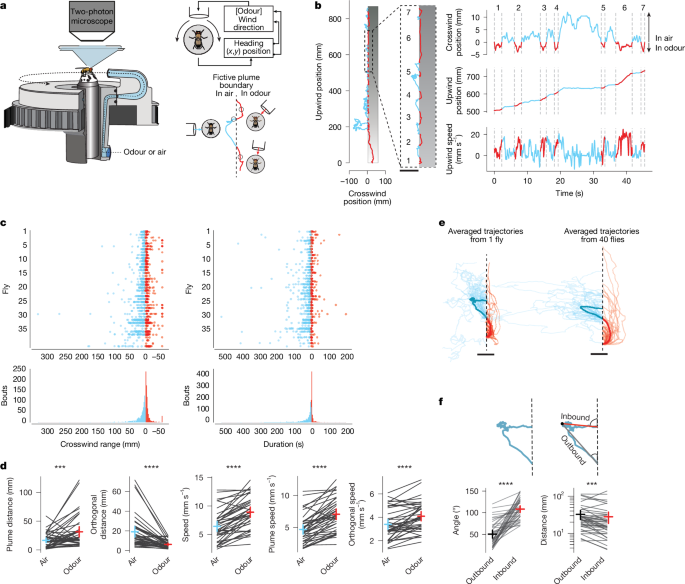
To construct average trajectories (Figs. 1e, 2e–h, 3f and 6j and Extended Data Figs. 5e, 6a and 7b), x and y coordinates for each outside or inside bout were upsampled to contain 10,000 points through linear interpolation between data points using the pandas library in Python. This allowed us to average x and y coordinates regardless of the length of the inside or outside bout. Upsampled x and y coordinates were averaged to produce one set of (x, y) coordinates for each fly. To construct an average across flies, the averages generated from individual flies were averaged together.

Entry and exit angles

Entry and exit angles were determined by calculating the mean travelling direction in the 0.5 s before and 0.5 s after crossing the plume’s boundary.

Analysis of inbound and outbound segments

The outside trajectories of flies tracking a vertical plume were simplified into straight-line segments using the Ramer–Douglas–Peucker (RDP) algorithm58, which simplifies a set of x, y coordinates by iteratively reducing the number of points in the trace. The parameter ε determines the maximum allowed distance between the simplified and original trajectories and was 1 mm. These trajectories were then averaged using the linear interpolation method described above providing a single average trajectory for each fly. From this average trajectory, ‘outbound’ (away from the edge) and ‘inbound’ (back towards the edge) path lengths were calculated as follows: (1) outbound path length was calculated as the path length from the point of exiting the plume to the farthest point orthogonal to the plume’s edge; and (2) inbound path length was calculated as the path length from the farthest point orthogonal to the plume’s edge back to the plume’s boundary. These three points—plume exit point, farthest point and plume entry point—define a triangle, the upwind angles of which define inbound and outbound angles as indicated in Fig. 1f. For analyses of simulated inbound and outbound trajectories in a random search model (Extended Data Fig. 5d,e), we took the total number of outside bouts for each fly and then randomly selected the same number of outside simulated outside trajectories. From this collection of random trajectories, we used the method above to generate an average trajectory and then calculated outbound and inbound lengths.

Definition of anemotaxis

Trajectories of flies before ACV exposure (pre-air period) were divided into anemotaxis bouts, defined in a similar manner to menotaxis bouts in a previous study6. Flies’ trajectories were simplified into straight-line segments using the Ramer–Douglas–Peucker algorithm (ε = 10 mm). Segments of length greater than 50 mm were assigned as anemotaxis bouts. See Fig. 6e,f.

Random-walk model

We simplified the outside trajectories of 40 flies tracking a vertical plume using the Ramer–Douglas–Peucker algorithm (ε = 1 mm) and extracted the straight-line distances (run lengths) that flies travelled between successive turns and the angles between consecutive straight-line vectors (turn angles) to capture the changes in heading direction. Run lengths and turn angles were each stored in a separate library. We simulated random-walk trajectories by randomly sampling from the two empirical distributions of run lengths and turn angles. Simulated flies started at the plume’s edge and the initial run length was assigned a heading that was drawn randomly from the initial segment heading directions from the plume (Extended Data Fig. 5b). At each step: (1) a run length was randomly sampled from the empirical distribution of run lengths; (2) a turn angle was randomly sampled from the empirical distribution of turn angles; and (3) the simulated fly moved forwards by the run length and then adjusted its heading by the turn angle.

The simulation continued until the simulated fly either re-encountered the plume edge or exceeded a maximum distance travelled of 500 mm in the direction perpendicular to the plume’s edge, which is the same maximum distance that flies were allowed to travel in experiments before a trial was terminated.

To reflect the natural tendency of flies to walk upwind even in the absence of odour cues16, we modified the random-walk model to include an upwind bias. We adjusted the turn direction on the basis of a sinusoidal probability function whose magnitude scaled between 0 and 1 (value a). When a = 0, the probability of turning left or right is the same for all heading directions. As the values of a increase from a = 0 to a = 1, the fly becomes progressively more biased to turn left when it is facing right, and to turn right when facing left. The value of a was selected to match that of real flies (Extended Data Fig. 5c), mirroring the upwind bias observed in actual flies outside the odour plume.

Given that random exploration outside the plume should not depend on the geometry of the plume tracked, the same model was used to simulate outside trajectories for flies tracking the 45°, 90° and jumping plumes, drawing from the same empirically derived libraries of run lengths and turn angles (Extended Data Fig. 5g–i). The only difference between the models was the initial heading, which was sampled from the initial segment heading directions for the 45° and 90° trajectories.

Functional imaging

All functional imaging experiments were performed on an Ultima or Investigator two-photon laser scanning microscope (Bruker) equipped with galvanometers driving a Chameleon Ultra II Ti:Sapphire laser. Emitted fluorescence was detected with GaAsP photodiode (Hamamatsu) detectors. Images were acquired with an Olympus 40×, 0.8 NA or 20×, 1.0 NA objective at 512 × 512 pixel resolution. The laser was tuned to 920 nm for all experiments. The out-of-objective power for all experiments was around 15 mW and never exceeded 25 mW. For volumetric imaging, three to five slices were recorded using a piezoelectric Z-focus (Bruker) at a rate of 3–10 Hz.

Data alignment

To align the imaging and behavioural data, we used a 3.3-V digital pulse from a RaspberryPi to initiate recording of an imaging stack through the PrairieView (Bruker) I/O interface. The RaspberryPi continued to send 3.3-V pulses every 10 s, which were recorded with PrairieView for confirmatory alignment of the imaging and behavioural data. Behavioural variables were captured at 60–61 frames per second, whereas neural activity (fluorescence) was captured at 3–10 frames per second. To align these two distinct time series, a standardized and regular time series was generated for each trace containing 100-ms time bins (0, 100, 200, 300 and so on). Behavioural data were binned at the centre of each time point and averaged. Imaging data were upsampled using linear interpolation at the same 100-ms time bins. Custom Python scripts were used to synchronize and log incoming FicTrac variables and outgoing MFC and motor commands, allowing us to align the wind direction, odour concentration, behavioural data and imaging frames.

Image registration and regions of interest

All images were stored as individual tiff files, which were registered using the StackReg function of the pystackreg library. Regions of interest were drawn using custom Python scripts, Fiji or a custom MATLAB GUI. To quantify EPG neuron activity recorded from the protocerebral bridge, we followed the methods described in a previous study35 and manually defined each of the 16 glomeruli from the registered stacks corresponding to each imaging plane.

FC2 neuron activity during edge tracking was recorded in the fan-shaped body. EPG neuron activity in the ellipsoid body was recorded synchronously to allow for direct comparison of their phase relationships during an experiment. To quantify FC2 neuron activity, we manually defined the lateral borders of the fan-shaped body, extended these lines down to a point and divided the arc defined by these intersecting lines into 16 wedges. Pixels were assigned to each wedge if they resided within the wedge and within the footprint of the FC2 neurons, defined by masks that were drawn manually in each imaging layer on the basis of their arborization pattern. To quantify EPG neuron activity recorded in the ellipsoid body, we divided the ellipsoid body radially into 16 sub-wedges from a manually defined centre. Pixels were assigned to each wedge if they resided within the wedge and within the footprint of the EPG neurons, defined by masks that were drawn manually in each imaging layer on the basis of their arborization pattern.

ΔF/F 0 values were determined by the formula (F − F 0 )/F 0 , where F is the mean pixel value within a wedge or glomerulus and F 0 is the mean of the lowest 10% of F values.

Neuronal phase analysis

Phase was determined by two methods. For recordings of EPG neurons in the protocerebral bridge, phase was calculated as described previously59. For each time point, the Fourier transform was taken on the ΔF/F 0 activity vector of the 16 glomeruli. Phase was determined as the phase of the Fourier spectrum at a period of 8, the peak periodicity of the power spectrum. For recordings of EPG neurons in the ellipsoid body and FC2 neurons in the fan-shaped body, phase was defined as the population vector average of wedge signals31,35. In summary, the 16 wedges of the ellipsoid body and fan-shaped body were assigned angles from −180° to 180°, equally dividing 360° of azimuthal space. Angles were assigned so that ellipsoid body and fan-shaped body wedges were in correspondence as per the connectome38. In the ellipsoid body, wedges were counted anticlockwise starting from the most ventral wedge to the right of the midline viewed from posterior to anterior. In the fan-shaped body, wedges were counted from right to left midline viewed from posterior to anterior. For each time point, each wedge was assigned a vector with length equal to the ΔF/F 0 value and direction given by its assigned angle. Phase was the angle of the population vector average of these vectors at each time point.

Phase nulling and bump amplitude assessment

Phase nulled EPG and FC2 signals were calculated as described previously35,59. At each frame, we rotated the signal by the estimated phase of the activity bump in that frame, such that all bumps were aligned. To compare EPG bumps recorded in the protocerebral bridge in and out of odour, we separated frames corresponding to when the fly was in or out of the odour and averaged 122 together with the signal from all these frames to get the average bump profile. The mean of phase-nulled FC2 and EPG bumps in Extended Data Fig. 14d was taken over a 0.5-s window before entries to the jumped plume and the preceding plume exit.

FC2 and EPG bump amplitude was assessed by two measures: the mean ΔF/F 0 across wedges and the population vector amplitude (PVA). Both measurements were taken over the same time period for the assessment of phase-nulled bumps. PVA was calculated as described previously6. The 16 wedges of the ellipsoid body and fan-shaped body were assigned activity-weighted vectors as for neuronal phase analysis (see above). PVA was calculated as the hypotenuse of the mean vector across wedges.

Phase calibration to allocentric coordinates

The anatomical locations of activity bumps in the central complex correspond to azimuthal orientations in allocentric space. However, the mapping from anatomical to external coordinates varies between individuals and can remap during an experiment31. To produce EPG and FC2 signals aligned to external coordinates, we rotated phase and wedges by an offset at each time point, such that phase angle 0° was aligned upwind and the central two wedges corresponded to 22.5° to the left and right of the upwind direction (Fig. 6d,e). The offset was the rolling mean (over 2 s) of the difference between the EPG phase and the fly’s heading, because the EPG signal provided a faithful neural correlate of heading relative to the wind (Fig. 3b–d). To rotate wedges, this offset was converted to an integer value varying between −8 and 8 by rounding to the nearest 22.5°. The same offset was applied to EPG and FC2 signals.

Model

Time discretization

We bin the data into time intervals of 0.2 s and run the behavioural model in discrete time steps with this same interval. Because we are modelling the motion of the fly, we exclude data points when the fly’s speed is less than 1 mm s−1.

Edge-crossing events for memory update

To avoid spurious events and to account for the finite width of the odour boundary, we define an edge crossing as when a fly is on one side of the odour boundary for three consecutive time points and then on the other side for three consecutive time points. We define the fly’s velocity unit vector at the time of the crossing, \(\hat{{\bf{v}}},\) as its velocity averaged over this five-time-step interval (1 s), normalized to unit length.

State

The model has two states: returning and leaving. When the fly leaves the odour plume in the leaving state, a time interval is drawn from a negative binomial distribution NB(r leave , 1 − p leave ) and, after that number of time steps, the state switches to the returning state if the fly is still out of the plume. When the fly enters the odour plume in the returning state, a time interval is drawn from a negative binomial distribution NB(r return , 1 − p return ) and, after that number of time steps, the state switches to the leaving state if the fly is still in the plume. Otherwise, no transitions occur. The parameters r leave , p leave , r return and p return are determined by fitting to data by the procedure described below.

Memory

The model stores 2D vector memories of plume exit and entry directions. The entry-memory vector m entry is updated at the time of each entry by

$${{\bf{m}}}_{\text{entry}}\leftarrow {a}_{\text{entry}}{{\bf{m}}}_{\text{entry}}+{b}_{\text{entry}}\hat{{\bf{v}}}+{{\boldsymbol{\epsilon }}}_{\text{entry}},$$

where \(\hat{{\bf{v}}}\) is the entry-velocity unit vector defined above, and the two components of ϵ entry are random variables drawn from a normal distribution with zero mean and variance \({{\sigma }}_{{\rm{entry}}}^{2}\). The exit memory vector m exit is updated at the time of each exit by

$${{\bf{m}}}_{\text{exit}}\leftarrow {a}_{\text{exit}}{{\bf{m}}}_{\text{exit}}+{b}_{\text{exit}}\hat{{\bf{v}}}+{{\boldsymbol{\epsilon }}}_{\text{exit}},$$

with \(\hat{{\bf{v}}}\) the exit-velocity unit vector and ϵ exit drawn from a normal distribution with zero mean and variance \({{\sigma }}_{{\rm{exit}}}^{2}\). In simulations, we ignore updates for which the exit \(\hat{{\bf{v}}}\) is more than 60° away from the upwind direction. This follows the intuition that flies have an innate tendency to exit upwind. Other than during these plume boundary crossings, m entry and m exit remain unchanged. For real flies, the values of the memory vectors at the beginning of a trajectory depend on unknown previous history. We therefore model m entry (0) as the null vector and m exit (0) with a trajectory-specific Gaussian prior N \(({{\boldsymbol{\mu }}}_{0},{\sigma }_{0}^{2}I)\) during fitting.

The parameters a entry , b entry , \({\sigma }_{{\rm{entry}}}^{2},\) a exit , b exit , \({\sigma }_{{\rm{exit}}}^{2}\), μ 0 and \({\sigma }_{0}^{2}\) are determined by the fitting procedure described below. During fitting, nonzero values of \({\sigma }_{0}^{2}\), \({\sigma }_{{\rm{entry}}}^{2}\) and \({\sigma }_{{\rm{exit}}}^{2}\) allow unexplained variation of latent memories. However, during simulation, we set \({\sigma }_{0}^{2}={\sigma }_{{\rm{entry}}}^{2}={\sigma }_{{\rm{exit}}}^{2}=0\) to test the effectiveness of our hypotheses without introducing extra noise into the memories. When simulating from models fitted to a single trajectory, as in Extended Data Fig. 8d, we set the initial exit memory to μ 0 . When simulating from the average fly model (parameters computed from multiple trajectories; Fig. 4b), we set the upwind component of the initial exit memory to a fixed value \({w}_{\parallel }\) equal to the median of the upwind components of μ 0 from all training trajectories, and we sample the crosswind component from a uniform distribution over the range from −2w ⊥ to +2w ⊥ , where w ⊥ is the median of the absolute value of the crosswind components of μ 0 from all training trajectories.

Velocity update

In the leaving state, velocity is updated at every time step with a decay term, a bias towards the current exit memory and a noise term,

$${\bf{v}}(t)={c}_{\text{leave}}{\bf{v}}(t-1)+{(1-c}_{\text{leave}}){{\bf{m}}}_{\text{exit}}+{{\boldsymbol{\xi }}}_{\text{leave}}(t),$$

with \({{\boldsymbol{\xi }}}_{\text{leave}}(t)\) drawn from a Gaussian distribution with zero mean and variance \({\sigma }_{\text{leave}}^{2}\). Similarly, in the returning state, the velocity update is

$${\bf{v}}(t)={c}_{\text{return}}{\bf{v}}(t-1)+{(1-c}_{\text{return}}){{\bf{m}}}_{\text{entry}}+{{\boldsymbol{\xi }}}_{\text{return}}(t),$$

with \({{\boldsymbol{\xi }}}_{\text{return}}(t)\) drawn from a Gaussian distribution with zero mean and variance \({\sigma }_{\text{return}}^{2}\). The parameters c leave , c return , \({\sigma }_{\text{leave}}^{2}\) and \({\sigma }_{\text{return}}^{2}\) are determined by the fitting procedure described below.

Variational inference and parameter learning

For each trajectory, we fitted a trajectory-specific model using a variational expectation-maximization procedure. In the variational E-step, we inferred the binary leaving and returning states z 1:T , entry memories m entry, 1:T and exit memories m exit ,1:T over the T time steps of the trajectory, while holding the model parameters fixed. Because the exact posterior p(z 1:T ,m entry ,1:T ,m exit,1:T |v 1:T ,o 1:T ) is intractable, where v 1:T denotes observed velocities and o 1:T denotes odour observations, we used the mean-field approximation q(z 1:T ,m entry ,1:T ,m exit,1:T ) = q(z 1:T )q(m entry ,1:T )q(m exit,1:T ), following a previous study41. We optimized this variational distribution by coordinate ascent on the evidence lower bound (ELBO). In the M-step, we updated the model parameters by maximizing the ELBO while holding the current variational distribution fixed. We alternated between these two steps until the ELBO converged. When reporting inferred memories from real fly trajectories (Figs. 4g and 5f and Extended Data Figs. 8h, 10f and 12d), we used the mean of trajectory-specific variational memory distributions q(m 1:T ).

State durations were modelled with negative binomial distributions NB(r, 1 − p), parameterized by r and p. For r > 1, q(z 1:T ) was represented over an expanded Markov chain, in which each behavioural state was augmented with r − 1 substates60. We then updated r and p for both leaving and returning states by fitting negative binomial distributions to state durations in samples from q(z 1:T ). For simplicity, we fixed r = 1 during all but the final iteration of the fitting algorithm.

For the average fly model, we fitted a single set of optimal parameters (except for μ 0 and \({\sigma }_{0}^{2}\), which are still trajectory specific) to latent variable distributions calculated using the above procedure from the 28 trajectories with no fewer than 30 returns (Extended Data Fig. 8c,h). We chose a relatively large threshold on the number of returns to provide a high number of data points for determining the memory update parameters.

Average fly model parameters (Extended Data Fig. 8c): w ∥ = 6.299 mm s−1; w ⊥ = 1.695 mm s−1; entry memory (a = 0.727, b = 0.437 mm s−1) and exit memory (a = 0.956, b = 0.482 mm/s); return after entry (r = 2, p = 0.505) and leave after exit (r = 1, p = 0.81); returning state (c = 0.733, σ = 3.23 mm s−1) and leaving state (c = 0.6, σ = 3.255 mm s−1).

Comparison with data

We remove odour changes lasting only one or two time steps from simulated trajectories before comparing to fly data, which matches the preprocessing procedure for fly data that removed odour changes lasting less than 0.5 s.

Dynamic plume analysis

Plume video

We used a previously recorded 3,600-frame video (4 min long) of a surface odour plume3,17 in two forms: one in the original scale, with the plume video sampled at 15 Hz and a spatial resolution of 0.74 mm per pixel, and another in an expanded scale stretched fivefold in both space and time, simulating an expanded video sampled at 3 Hz with a spatial resolution of 3.7 mm per pixel. Because the edge tracking model depends on binary odour states, we binarized the odour signal with a threshold of 0.1 to assure sufficient odour encounters while preserving the turbulent properties at the downwind end of the plume, allowing us to explore how the model performs with different degrees of turbulence (Extended Data Fig. 13b).

Model simulations and threshold for success

We used the average fly model to simulate 2,000 trajectories for each dynamic plume type. For the unscaled plume, we set the simulation time step to 1/15 s (the frame rate of the video) and converted model parameters accordingly. We initialized trajectories uniformly within a 200 mm × 100-mm rectangular region spanning 100–300 mm downwind of the source and −60 to 40 mm in the crosswind direction, to assess how tracking success depends on the initial position within the plume. A trial was considered a success if the minimum distance of the simulated trajectory to the source was less than 20 mm. For the scaled plume, we set the simulation time step to 0.2 s, as in edge-tracking simulations, and we used the video frame closest in time at each step. We initialized trajectories uniformly within a 1,000 mm × 500-mm rectangular region spanning 500–1,500 mm downwind of the source and −300 to 200 mm in the crosswind direction. For the scaled plume, a trial was considered a success if the minimum distance to the source was less than 50 mm.

Effective entries and exits in dynamic plumes

Effective entry and exit events during simulation were defined over a 1-s interval (entry: 0.5 s odour off, 0.5 s odour on; exit: 0.5 s odour on, 0.5 s odour off), to be consistent with memory updating in edge-crossing events (plotted in Fig. 5b,e and Extended Data Fig. 13g). When comparing models with and without entry memory, we included only trajectories with at least one effective entry. For the unscaled plume, we further excluded trajectories for which the first effective entry was within a 20-mm alongwind distance from the source, yielding 1,593 out of 2,000 trials. For the scaled plume, we further excluded trajectories for which the first effective entry was within a 50 mm alongwind distance from the source, yielding 1,850 out of 2,000 trials.

Entry-memory crosswind predictivity

We denote \({\hat{{\bf{m}}}}_{\mathrm{entry}}={({m}_{\perp },{m}_{\parallel })}^{T}\) as the entry-memory vector normalized to unit length and \(\hat{{\bf{v}}}={({v}_{\perp },{v}_{\parallel })}^{T}\) as the entry-velocity unit vector. Crosswind predictivity is calculated as the product of m ⊥ and v ⊥ at the time of each entry.

Statistics and reproducibility

Data were processed and analysed using custom scripts written in Python and MATLAB. No statistical methods were used to predetermine sample sizes; sample sizes were selected on the basis of common practice in the field and were comparable with those used in previous studies. No randomization of experimental sessions and no blinding to experimental conditions were used during data collection or analysis. The principal behavioural finding—that flies track odour plumes by repeatedly exiting and returning to the plume boundary (edge tracking)—was highly reproducible across flies, experimental paradigms and experimenters. Unless otherwise stated, all statistical comparisons were performed using two-tailed non-parametric tests. Statistical details, including sample sizes, statistical tests and exact P values, are provided in the corresponding figure legends or Supplementary Table 1.

Reporting summary

Further information on research design is available in the Nature Portfolio Reporting Summary linked to this article.